Convolutional Neural Networks (LeNet)
:label:sec_lenet
We now have all the ingredients required to assemble
a fully-functional convolutional neural network.
In our first encounter with image data,
we applied a multilayer perceptron (:numref:sec_mlp_scratch)
to pictures of clothing in the Fashion-MNIST dataset.
To make this data amenable to multilayer perceptrons,
we first flattened each image from a $28\times28$ matrix
into a fixed-length $784$-dimensional vector,
and thereafter processed them with fully-connected layers.
Now that we have a handle on convolutional layers,
we can retain the spatial structure in our images.
As an additional benefit of replacing dense layers with convolutional layers,
we will enjoy more parsimonious models (requiring far fewer parameters).
In this section, we will introduce LeNet, among the first published convolutional neural networks to capture wide attention for its performance on computer vision tasks. The model was introduced (and named for) Yann Lecun, then a researcher at AT&T Bell Labs, for the purpose of recognizing handwritten digits in images LeNet5. This work represented the culmination of a decade of research developing the technology. In 1989, LeCun published the first study to successfully train convolutional neural networks via backpropagation.
At the time LeNet achieved outstanding results matching the performance of Support Vector Machines (SVMs), then a dominant approach in supervised learning. LeNet was eventually adapted to recognize digits for processing deposits in ATM machines. To this day, some ATMs still run the code that Yann and his colleague Leon Bottou wrote in the 1990s!
LeNet
At a high level, LeNet consists of three parts:
(i) a convolutional encoder consisting of two convolutional layers; and
(ii) a dense block consisting of three fully-connected layers;
The architecture is summarized in :numref:img_lenet.

:label:img_lenet
The basic units in each convolutional block are a convolutional layer, a sigmoid activation function, and a subsequent average pooling operation. Note that while ReLUs and max-pooling work better, these discoveries had not yet been made in the 90s. Each convolutional layer uses a $5\times 5$ kernel and a sigmoid activation function. These layers map spatially arranged inputs to a number of 2D feature maps, typically increasing the number of channels. The first convolutional layer has 6 output channels, while th second has 16. Each $2\times2$ pooling operation (stride 2) reduces dimensionality by a factor of $4$ via spatial downsampling. The convolutional block emits an output with size given by (batch size, channel, height, width).
In order to pass output from the convolutional block to the fully-connected block, we must flatten each example in the minibatch. In other words, we take this 4D input and transform it into the 2D input expected by fully-connected layers: as a reminder, the 2D representation that we desire has uses the first dimension to index examples in the minibatch and the second to give the flat vector representation of each example. LeNet's fully-connected layer block has three fully-connected layers, with 120, 84, and 10 outputs, respectively. Because we are still performing classification, the 10-dimensional output layer corresponds to the number of possible output classes.
While getting to the point where you truly understand
what is going on inside LeNet may have taken a bit of work,
hopefully the following code snippet will convince you
that implementing such models with modern deep learning libraries
is remarkably simple.
We need only to instantiate a Sequential Block
and chain together the appropriate layers.
%load ../utils/djl-imports
%load ../utils/plot-utils
import ai.djl.basicdataset.cv.classification.*;
import ai.djl.metric.*;
import org.apache.commons.lang3.ArrayUtils;
Engine.getInstance().setRandomSeed(1111);

NDManager manager = NDManager.newBaseManager();

SequentialBlock block = new SequentialBlock();

block
    .add(Conv2d.builder()
                .setKernelShape(new Shape(5, 5))
                .optPadding(new Shape(2, 2))
                .optBias(false)
                .setFilters(6)
                .build())
    .add(Activation::sigmoid)
    .add(Pool.avgPool2dBlock(new Shape(5, 5), new Shape(2, 2), new Shape(2, 2)))
    .add(Conv2d.builder()
                .setKernelShape(new Shape(5, 5))
                .setFilters(16).build())
    .add(Activation::sigmoid)
    .add(Pool.avgPool2dBlock(new Shape(5, 5), new Shape(2, 2), new Shape(2, 2)))
    // Blocks.batchFlattenBlock() will transform the input of the shape (batch size, channel,
    // height, width) into the input of the shape (batch size,
    // channel * height * width)
    .add(Blocks.batchFlattenBlock())
    .add(Linear
                .builder()
                .setUnits(120)
                .build())
    .add(Activation::sigmoid)
    .add(Linear
                .builder()
                .setUnits(84)
                .build())
    .add(Activation::sigmoid)
    .add(Linear
                .builder()
                .setUnits(10)
                .build());
We took a small liberty with the original model, removing the Gaussian activation in the final layer. Other than that, this network matches the original LeNet5 architecture. We also create the Model and Trainer object so that we initialize the structure once.
By passing a single-channel (black and white)
$28 \times 28$ image through the net
and printing the output shape at each layer,
we can inspect the model to make sure
that its operations line up with
what we expect from :numref:img_lenet_vert.
float lr = 0.9f;
Model model = Model.newInstance("cnn");
model.setBlock(block);

Loss loss = Loss.softmaxCrossEntropyLoss();

Tracker lrt = Tracker.fixed(lr);
Optimizer sgd = Optimizer.sgd().setLearningRateTracker(lrt).build();

DefaultTrainingConfig config = new DefaultTrainingConfig(loss).optOptimizer(sgd) // Optimizer (loss function)
        .optDevices(Engine.getInstance().getDevices(1)) // Single GPU
        .addEvaluator(new Accuracy()) // Model Accuracy
        .addTrainingListeners(TrainingListener.Defaults.basic());

Trainer trainer = model.newTrainer(config);

NDArray X = manager.randomUniform(0f, 1.0f, new Shape(1, 1, 28, 28));
trainer.initialize(X.getShape());

Shape currentShape = X.getShape();

for (int i = 0; i < block.getChildren().size(); i++) {
    Shape[] newShape = block.getChildren().get(i).getValue().getOutputShapes(new Shape[]{currentShape});
    currentShape = newShape[0];
    System.out.println(block.getChildren().get(i).getKey() + " layer output : " + currentShape);
}
Note that the height and width of the representation at each layer throughout the convolutional block is reduced (compared to the previous layer). The first convolutional layer uses $2$ pixels of padding to compensate for the the reduction in height and width that would otherwise result from using a $5 \times 5$ kernel. In contrast, the second convolutional layer foregoes padding, and thus the height and width are both reduced by $4$ pixels. As we go up the stack of layers, the number of channels increases layer-over-layer from 1 in the input to 6 after the first convolutional layer and 16 after the second layer. However, each pooling layer halves the height and width. Finally, each fully-connected layer reduces dimensionality, finally emitting an output whose dimension matches the number of classes.

:label:img_lenet_vert
Data Acquisition and Training
Now that we have implemented the model, let's run an experiment to see how LeNet fares on Fashion-MNIST.
int batchSize = 256;
int numEpochs = Integer.getInteger("MAX_EPOCH", 10);
double[] trainLoss;
double[] testAccuracy;
double[] epochCount;
double[] trainAccuracy;

epochCount = new double[numEpochs];

for (int i = 0; i < epochCount.length; i++) {
    epochCount[i] = (i + 1);
}

FashionMnist trainIter = FashionMnist.builder()
        .optUsage(Dataset.Usage.TRAIN)
        .setSampling(batchSize, true)
        .optLimit(Long.getLong("DATASET_LIMIT", Long.MAX_VALUE))
        .build();


FashionMnist testIter = FashionMnist.builder()
        .optUsage(Dataset.Usage.TEST)
        .setSampling(batchSize, true)
        .optLimit(Long.getLong("DATASET_LIMIT", Long.MAX_VALUE))
        .build();

trainIter.prepare();
testIter.prepare();
While convolutional networks have few parameters, they can still be more expensive to compute than similarly deep multilayer perceptrons because each parameter participates in many more multiplications. If you have access to a GPU, this might be a good time to put it into action to speed up training.
The training function trainingChapter6 is also similar
to trainChapter3 defined in :numref:sec_softmax_scratch.
Since we will be implementing networks with many layers
going forward, we will rely primarily on DJL.
The following train function assumes a DJL model
as input and is optimized accordingly.
We initialize the model parameters
on the block using the Xavier initializer.
Just as with MLPs, our loss function is cross-entropy,
and we minimize it via minibatch stochastic gradient descent.
public void trainingChapter6(ArrayDataset trainIter, ArrayDataset testIter,
             int numEpochs, Trainer trainer) throws IOException, TranslateException {

    double avgTrainTimePerEpoch = 0;
    Map<String, double[]> evaluatorMetrics = new HashMap<>();

    trainer.setMetrics(new Metrics());

    EasyTrain.fit(trainer, numEpochs, trainIter, testIter);

    Metrics metrics = trainer.getMetrics();

    trainer.getEvaluators().stream()
        .forEach(evaluator -> {
            evaluatorMetrics.put("train_epoch_" + evaluator.getName(), metrics.getMetric("train_epoch_" + evaluator.getName()).stream()
                    .mapToDouble(x -> x.getValue().doubleValue()).toArray());
            evaluatorMetrics.put("validate_epoch_" + evaluator.getName(), metrics.getMetric("validate_epoch_" + evaluator.getName()).stream()
                    .mapToDouble(x -> x.getValue().doubleValue()).toArray());
        });

    avgTrainTimePerEpoch = metrics.mean("epoch");

    trainLoss = evaluatorMetrics.get("train_epoch_SoftmaxCrossEntropyLoss");
    trainAccuracy = evaluatorMetrics.get("train_epoch_Accuracy");
    testAccuracy = evaluatorMetrics.get("validate_epoch_Accuracy");

    System.out.printf("loss %.3f," , trainLoss[numEpochs-1]);
    System.out.printf(" train acc %.3f," , trainAccuracy[numEpochs-1]);
    System.out.printf(" test acc %.3f\n" , testAccuracy[numEpochs-1]);
    System.out.printf("%.1f examples/sec \n", trainIter.size() / (avgTrainTimePerEpoch / Math.pow(10, 9)));
}
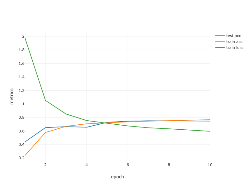
Now let us train the model.
trainingChapter6(trainIter, testIter, numEpochs, trainer);
String[] lossLabel = new String[trainLoss.length + testAccuracy.length + trainAccuracy.length];

Arrays.fill(lossLabel, 0, trainLoss.length, "train loss");
Arrays.fill(lossLabel, trainAccuracy.length, trainLoss.length + trainAccuracy.length, "train acc");
Arrays.fill(lossLabel, trainLoss.length + trainAccuracy.length,
                trainLoss.length + testAccuracy.length + trainAccuracy.length, "test acc");

Table data = Table.create("Data").addColumns(
    DoubleColumn.create("epoch", ArrayUtils.addAll(epochCount, ArrayUtils.addAll(epochCount, epochCount))),
    DoubleColumn.create("metrics", ArrayUtils.addAll(trainLoss, ArrayUtils.addAll(trainAccuracy, testAccuracy))),
    StringColumn.create("lossLabel", lossLabel)
);

render(LinePlot.create("", data, "epoch", "metrics", "lossLabel"), "text/html");
Summary
- A ConvNet is a network that employs convolutional layers.
- In a ConvNet, we interleave convolutions, nonlinearities, and (often) pooling operations.
- These convolutional blocks are typically arranged so that they gradually decrease the spatial resolution of the representations, while increasing the number of channels.
- In traditional ConvNets, the representations encoded by the convolutional blocks are processed by one (or more) dense layers prior to emitting output.
- LeNet was arguably the first successful deployment of such a network.
Exercises
- Replace the average pooling with max pooling. What happens?
- Try to construct a more complex network based on LeNet to improve its accuracy.
- Adjust the convolution window size.
- Adjust the number of output channels.
- Adjust the activation function (ReLU?).
- Adjust the number of convolution layers.
- Adjust the number of fully connected layers.
- Adjust the learning rates and other training details (initialization, epochs, etc.)
- Try out the improved network on the original MNIST dataset.
- Display the activations of the first and second layer of LeNet for different inputs (e.g., sweaters, coats).