Notebook

[MCB 32L]: Introduction to Python¶

Professor Robin Ball¶

We will introduce you to data analysis using Python and Jupyter notebooks, which you will use in other labs this semester.

Estimated Time: ~1 Hour

Table of Contents¶

Intro to Jupyter notebooks

Introduction to Python

a Entering and Naming your data

b Basic calculations
Graphing with matplotlib
Graphing reaction time data

Welcome to Jupyter ¶

Welcome to the Jupyter Notebook! Notebooks are documents that can contain text, code, visualizations, and more. We'll be using them in this lab to manipulate and visualize our data.

A notebook is composed of rectangular sections called cells. There are two kinds of cells: markdown and code. A markdown cell, such as this one, contains text. A code cell contains code in Python, a programming language that we will be using for the remainder of this module. You can select any cell by clicking it once. After a cell is selected, you can navigate the notebook using the up and down arrow keys.

To run a code cell once it's been selected,

press Shift-Enter, or
click the Run button in the toolbar at the top of the screen.

If a code cell is running, you will see an asterisk (*) appear in the square brackets to the left of the cell. Once the cell has finished running, a number will replace the asterisk and any output from the code will appear under the cell.

In [ ]:

# run this cell
print("Hello World!")

You'll notice that many code cells contain lines of blue text that start with a #. These are comments. Comments often contain helpful information about what the code does or what you are supposed to do in the cell. The leading # tells the computer to ignore them.

In [ ]:

# this is a comment- running the cell will do nothing!

Code cells can be edited any time after they are highlighted. Try editing the next code cell to print your name.

In [ ]:

# edit the code to print your name
print("Hello: my name is (name)")

Saving and Loading¶

Your notebook can record all of your text and code edits, as well as any graphs you generate or calculations you make. You can save the notebook in its current state by clicking Control-S, clicking the floppy disc icon in the toolbar at the top of the page, or by going to the File menu and selecting "Save and Checkpoint".

The next time you open the notebook, it will look the same as when you last saved it.

Note: after loading a notebook you will see all the outputs (graphs, computations, etc) from your last session, but you won't be able to use any variables you assigned or functions you defined. You can get the functions and variables back by re-running the cells where they were defined- the easiest way is to highlight the cell where you left off work, then go to the Cell menu at the top of the screen and click "Run all above". You can also use this menu to run all cells in the notebook by clicking "Run all".

Completing the Notebooks¶

QUESTION cells are in blue and ask you to enter in lab data, make graphs, or do other lab tasks. To receive full credit for your lab, you must complete all QUESTION cells and run all the code.

1. Python ¶

Python is programming language- a way for us to communicate with the computer and give it instructions. Just like any language, Python has a vocabulary made up of words it can understand, and a syntax giving the rules for how to structure communication.

Python doesn't have a large vocabulary or syntax, but it can be used for many, many computational tasks.

Bits of communication in Python are called expressions- they tell the computer what to do with the data we give it.

Here's an example of an expression.

In [ ]:

# an expression
14 + 20

When you run the cell, the computer evaluates the expression and prints the result. Note that only the last line in a code cell will be printed, unless you explicitly tell the computer you want to print the result.

In [ ]:

# more expressions. what gets printed and what doesn't?
100 / 10

print(4.3 + 10.98)

33 - 9 * (40000 + 1)

884

Many basic arithmetic operations are built in to Python, like * (multiplication), + (addition), - (subtraction), and / (division). There are many others, which you can find information about here.

The computer evaluates arithmetic according to the PEMDAS order of operations (just like you probably learned in middle school): anything in parentheses is done first, followed by exponents, then multiplication and division, and finally addition and subtraction.

In [ ]:

# before you run this cell, can you say what it should print?
4 - 2 * (1 + 6 / 3)

A Note on Errors ¶

Python is a language, and like natural human languages, it has rules. It differs from natural language in two important ways:

The rules are simple. You can learn most of them in a few weeks and gain reasonable proficiency with the language in a semester.
The rules are rigid. If you're proficient in a natural language, you can understand a non-proficient speaker, glossing over small mistakes. A computer running Python code is not smart enough to do that.

Whenever you write code, you'll make mistakes. When you run a code cell that has errors, Python will sometimes produce error messages to tell you what you did wrong.

Errors are normal; experienced programmers see errors all the time. When you make an error, you just have to find the source of the problem, fix it, and move on.

We have made an error in the next cell. Delete the #, then run it and see what happens.

In [ ]:

# print("This line is missing something."

You should see something like this (minus our annotations):

Error Image

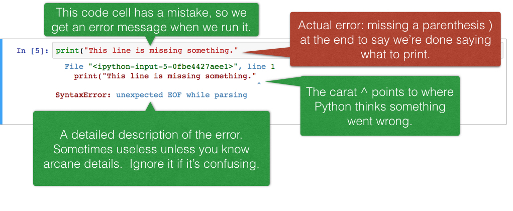
The last line of the error output attempts to tell you what went wrong. The syntax of a language is its structure, and this SyntaxError tells you that you have created an illegal structure. "EOF" means "end of file," so the message is saying Python expected you to write something more (in this case, a right parenthesis) before finishing the cell.

There's a lot of terminology in programming languages, but you don't need to know it all in order to program effectively. If you see a cryptic message like this, you can often get by without deciphering it. (Of course, if you're frustrated, you can usually find out by searching for the error message online or asking course staff for help).

1a. Entering and Naming your data ¶

Sometimes, the values you work with can get cumbersome- maybe the expression that gives the value is very complicated, or maybe the value itself is long. In these cases it's useful to give the value a name.

We can name values using what's called an assignment statement.

In [ ]:

# assigns 442 to x
x = 442

The assignment statement has three parts. On the left is the name (x). On the right is the value (442). The equals sign in the middle tells the computer to assign the value to the name.

You'll notice that when you run the cell with the assignment, it doesn't print anything. But, if we try to access x again in the future, it will have the value we assigned it.

In [ ]:

# show the value of x
x

You can also assign names to expressions. The computer will compute the expression and assign the name to the result of the computation.

In [ ]:

y = 50 * 2 + 1
y

We can then use these names as if they were whatever they stand for (in this case, numbers).

In [ ]:

x - 42

In [ ]:

x + y

Lists¶

In Python, you can also make lists of numbers. A Python list is enclosed in square brackets. Items inside the list are separated by commas.

In [ ]:

# a list
[7.0, 6.24, 9.98, 4]

Lists can have names too, which is handy for when you want to want to save a set of items without writing them out over and over again.

In [ ]:

my_list = [4, 8, 15, 16, 23, 42]
my_list

1b. Basic calculations ¶

Once you have your data in a list, Python has a variety of functions that can be used to perform calculations and draw conclusions.

Built-in functions¶

The most basic functions are built into Python. This means that Python already knows how to perform these functions without you needing to define them or import a library of functions. The print() function you saw earlier is an example of a built-in function. A full list of all built-in Python functions can be found here.

Below are a few examples of functions you may find useful during this class

In [ ]:

# what do you think this function calculates?
min(my_list)

In [ ]:

# what about this one?
max(my_list)

In this example, we passed a single list to each of the functions. However, you can also pass multiple numbers separated by commas, or even multiple lists! You can try it out below and see if you can figure out how Python is choosing which list is greater than the other.

In [ ]:

max([1, 2, 3], [3, 2, 0])

Some functions have optional arguments. For instance, the most basic usage of the round() function takes a single argument.

In [ ]:

round(3.14159)

You can also specify a second argument, which specifies how many decimal places you would like the output to have. If you don't include this argument, Python uses the default, which is zero.

In [ ]:

round(3.14159, 2)

`numpy`¶

For more complex calculations, you will need to either define functions or import functions that someone else has written. For numerical calculations, numpy is a popular library containing a wide variety of functions. If you are curious about all of the functions in the library, the numpy documentation can be found here.

In order to use these functions, you have to first run an import statement. Import statements for all required libraries are typically run at the beginning of a notebook.

In [ ]:

# This gives numpy an abbbreviation so that when we refer to it later we don't need to write the whole name out.
# We could abbreviate it however we want, but np is the conventional abbreviation for numpy.
import numpy as np

Now you can use all the functions in the numpy library. When using these functions, you must prefix them with np. so that Python knows to look in the numpy library for the function.

In [ ]:

np.mean(my_list)

2. Graphing with `matplotlib` ¶

The matplotlib library includes a variety of functions that allow us to build plots of data. Once again, you must first import the library before you can use it.

In [ ]:

# Import the library
import matplotlib.pyplot as plt

# This line allows the plots display to nicely in the notebook.
%matplotlib inline

Before you can use the plotting functions, you must first have some data to plot. Below are some data on Berkeley restaurants taken from Yelp.

In [ ]:

restaurants = ["Gypsy's", "Tacos Sinaloa", "Sliver", "Muracci's", "Brazil Cafe", "Thai Basil"]
rating = [4, 4, 4, 3.5, 4.5, 3.5]
number_of_ratings = [1666, 347, 1308, 294, 1246, 904]

You may be interested in seeing if there is a relationship between the number of ratings a restaurant has and their rating out 5 stars. It is difficult to determine this from looking at the numbers directly, so a plot can come in handy.

In [ ]:

# create a scatter plot
plt.scatter(number_of_ratings, rating)

# show the plot
plt.show()

Out of context, this plot is not very helpful because it doesn't have axis labels or a title. These components can be added using other matplotlib functions.

In [ ]:

# create a scatter plot
plt.scatter(number_of_ratings, rating)

# add the x-axis label
plt.xlabel("Number of Ratings")

# add the y-axis label
plt.ylabel("Star Rating (out of 5)")

# add a title
plt.title("Berkeley Restaurant Star Ratings by Number of Ratings")

# show the plot
plt.show()

There are many other attributes you can add to plots and many more types of plots you can create using this library. For a comprehensive description, visit the documentation! Included here are some basic plots that you may find useful for this class.

In [ ]:

# create a bar plot
plt.bar(restaurants, number_of_ratings)

# add the x-axis label
plt.xlabel("Restaurant")

# add the y-axis label
plt.ylabel("Number of Ratings")

# add a title
plt.title("Berkeley Restaurant Star Ratings")

# show the plot
plt.show()

In [ ]:

# create a histogram
plt.hist(rating)

# add the x-axis label
plt.xlabel("Star Rating (out of 5)")

# add the y-axis label
plt.ylabel("Frequency")

# add a title
plt.title("Berkeley Restaurant Star Rating Frequencies")

# show the plot
plt.show()

It is also possible to overlay multiple lines on a single plot. Below are some made up data about the number of people with each height in two different classes.

In [ ]:

height = [60, 61, 62, 63, 64, 65, 66, 67, 68, 69, 70, 71, 72]
class_one = [1, 1, 0, 3, 7, 4, 3, 7, 8, 3, 1, 2, 1]
class_two = [0, 0, 3, 1, 3, 4, 1, 2, 6, 2, 8, 5, 2]

You can use the .plot() function to plot both of these functions as line plots. If you run multiple calls to plotting functions in the same cell, Python will simply layer the resulting plots on the same plot.

In [ ]:

# create a line plot for the first class
# label this line as class one for the legend
plt.plot(height, class_one, label = "class one")

# create a line plot for the second class
# label this line as class two for the legend
plt.plot(height, class_two, label = "class two")

# add the x-axis label
plt.xlabel("Height (in)")

# add the y-axis label
plt.ylabel("Frequency")

# add the legend
plt.legend()

# add the title
plt.title("Frequencies of Different Heights for Two Classes")

# show the plot
plt.show()

3. Graphing reaction time data ¶

Now you will have a chance to make a graph with the reaction time data you collected during your lab. We will go over two different ways of entering your data.

3a. Using a list to enter data¶

QUESTION: Fill in the '...' with a list containing the reaction time values (in milliseconds) you recorded during lab.

In [ ]:

visual_reaction_time = [...]
auditory_reaction_time = [...]

Let's make a table from our two lists. Note that we enter the name of the column followed by the name of the list we want to put into that column.

In [ ]:

#Run this cell to import the function to make a table

from datascience import *

In [ ]:

Reaction_time_table = Table().with_columns("Visual reaction time", visual_reaction_time, "Auditory reaction time", auditory_reaction_time)
Reaction_time_table

Now you will take the mean of these data in order to create your bar plot. We will use the function np.mean().

QUESTION: Pass your lists to np.mean below so that the means are saved to the variables visual_reaction_time_mean and auditory_reaction_time_mean. You do not need to type in the numbers again, because you already assigned a name to each list. Put that name into the np.mean().

In [ ]:

visual_reaction_time_mean = ...
auditory_reaction_time_mean = ...

print(visual_reaction_time_mean)
print(auditory_reaction_time_mean)

Next, you will need to consider what type of graph is most suited to your data. Then, use the plotting functions you have just learned to create a plot of the data. Don't forget to add informative labels!

QUESTION: Create a bar plot of your data. Label your axes and remember to include units for the reaction times. You can copy the correct commands for labeling the axes from the graphs you made above. Just change the specific name for the axes.

Hint: Create two lists, one with the names of the variables (what will be on the x-axis) and another with the means you want to graph, and then pass those lists to plt.bar(). Again, you don't need to write in the numerical means, because you gave each mean a name in the cell above. The number for the visual reaction time mean is stored in the variable "visual_reaction_time_mean".

In [ ]:

# create two lists and then a bar plot from those lists
names = [...,...]
means = [...,...]
plt.bar(names, means)

# add the x-axis label

# add the y-axis label

# add a title

# show the plot
plt.show()

3b. Using a table to enter data¶

If you have a lot of data to enter, it might be easier to type it into an already existing grid, rather than writing all the numbers as a list. You will make a table of your reaction time data using this method.

QUESTION: Run the cell below to make the blank grid. Then replace the 0 values with your reaction time data. You can use the Tab key to move quickly between cells. Note that if you enter your data and then re-run the cell below, it will go back to zeroes and you will have to enter the numbers again.

In [ ]:

from table import *

reaction_time_table = make_table(rows = 5, cols = 3, 
                                 labels = ["Trial number", "Visual reaction time (ms)", "Auditory reaction time (ms)"], 
                                 types = ["integer", "decimal", "decimal"],
                                 values = {"Trial number" : ["1", "2", "3", "4", "5"]})

In [ ]:

reaction_time_table

You will get more practice working with tables and graphing data from tables in future labs, so we will end here.

In future labs, you will primarily use the make_table method, but if you do not like that method remember that you can also enter the data as lists.

You have just created your first plot! In the future, you can use this lab as a reference for Python basics and how to create simple graphs.

Saving the Notebook as an html file¶

Congrats on finishing your first lab notebook! To turn in this lab assignment follow the steps below:

Go to the File menu
Go to 'Save and Export Notebook As'
Select HTML
You will upload the html file into the bCourses assignment

If you also want to create a pdf version of the file for your records, follow these instructions:

Press Control + P (or Command + P on Mac) to open the Print preview
Change the destination so that it saves locally on your own computer.
Save as PDF
If you are stuck, follow further instructions here.

References¶

Sections of "Intro to Jupyter", adapted from materials by Kelly Chen and Ashley Chien in UC Berkeley Data Science Modules core resources
"A Note on Errors" subsection and "error" image adapted from materials by Chris Hench and Mariah Rogers for the Medieval Studies 250: Text Analysis for Graduate Medievalists data science module.
"Intro to Jupyter" and "Intro to Python" adapted from materials by Keeley Takimoto for the Berkeley Executive Education Program on Data Science and Analytics Module

Notebook developed by: Monica Wilkinson and Alex Nakagawa

Data Science Modules: http://data.berkeley.edu/education/modules

[MCB 32L]: Introduction to Python¶

Professor Robin Ball¶

Table of Contents¶

Welcome to Jupyter ¶

Saving and Loading¶

Completing the Notebooks¶

1. Python ¶

A Note on Errors ¶

1a. Entering and Naming your data ¶

Lists¶

1b. Basic calculations ¶

Built-in functions¶

numpy¶

2. Graphing with matplotlib ¶

3. Graphing reaction time data ¶

3a. Using a list to enter data¶

3b. Using a table to enter data¶

Saving the Notebook as an html file¶

References¶

`numpy`¶

2. Graphing with `matplotlib` ¶