Julia lang definition of plain-knit yarns ¶
Recently, K Crane defined 3d curves to model yarns and fibers for simple knitting.
We reproduce the plots from K Crane's paper, https://www.cs.cmu.edu/~kmcrane/Projects/Other/YarnCurve.pdf, taking the advantage of Julia, over C programming language, to write a more compact code, and moreover to plot the graphical objects directly, without involving an external library. Notice that automatic derivation (via ForwardDiff.jl) of vector valued functions $t\mapsto γ(t)$, $t\mapsto\dot{γ}(t)$, substantially reduces the lines of code, compared to the C version.
The yarns are represented as tubular surfaces, having as directrice a 3d curve, $t\to\gamma(t)\in\mathbb{R}^3$. To get the tube parameterizaion we implement the A. Hanson's algorithm, presented in Visualizing Quaternions, Morgan Kaufmann, 2006:
import ForwardDiff.derivative
import LinearAlgebra: norm, cross
import Rotations.UnitQuaternion
using  PlotlyJS
dγ(t)=derivative(γ, t) # t->̇γ(t)
ddγ(t)=derivative(dγ, t) #t->̈γ(t)

#get the tubular surface  parameterization:
function tube(γ::T, u::S, v::S; radius=0.1) where {S<:Real, T<:Function}
    tang = dγ(u)   #tangent(γ, u)
    ~iszero(tang) || error("null tangent vector!")
    unittan = tang/norm(tang)
    θ = acos(unittan[1])/2
    crossp= [0, -unittan[3], unittan[2]]  # cross product [1,0,0] x unittan
    quvect = sin(θ)*crossp/norm(crossp) #3-vector to define the quaternion
                                          #q=(cos(θ), sin(θ)*unitvect)
    q = isapprox(θ, π/2) ? UnitQuaternion(0, 0, 1, 0) : isapprox(θ, 0) ?
                   UnitQuaternion(1, 0 , 0, 0) : UnitQuaternion(cos(θ), quvect...)
    _, n₁, n₂,   = eachcol(q)
    return γ(u) + radius*cos(v) * n₁ + radius*sin(v) * n₂
end

#define  a fiber curve  parameterization (§3.2 Fiber Curves in K Crane's paper)
function fiber_curve(γ::T₁;
                     ω=4, r=0.5, Φ=0) where {T₁}  #, T₂, T₃<:Function
    # curve is t->γ(t), dγ: t->̇γ(t), ddγ: t->̈γ(t)
    θ(t) =  ω*t −2cos(t)+Φ
    unittan(t) = dγ(t)/norm(dγ(t))
    unitacc(t) = ddγ(t)/norm(ddγ(t))
    n₂(t) = cross(unittan(t), unitacc(t))  #binormal
    n₁(t) = cross(n₂(t), unittan(t))  #principal normal
    t->γ(t) + r*cos(θ(t)) * n₁(t) + r*sin(θ(t)) * n₂(t)
end
Define the PlotlyJS type data for plotting yarns and fibers:
burgundy = [[0, "#e26152"], [1, "#e26152"]] #kind of burgundy color
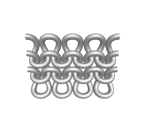
silver = [[0, "#bebebe"], [1.0, "#bebebe"]] #silver color
function surf(x::Matrix{T} , y::Matrix{T}, z::Matrix{T}; colorscale=burgundy) where T<:Real
surface(x=x, y=y, z=z, hoverinfo="skip",
colorscale=colorscale,
showscale=false,
lighting=attr(ambient=0.45,
diffuse=0.35,
fresnel=0.5,
specular=0.25,
roughness=0.45),
lightposition=attr(x=100,
y=100,
z=100
))
end
axes_off(fig)=
relayout!(fig, scene =attr(xaxis_visible=false,
yaxis_visible=false,
zaxis_visible=false))
function plot_data(traces)
fig = Plot(traces,
Layout(width=450, height=450,
#margin=attr(t=2, r=2, b=2, l=2),
scene=attr(aspectmode="data",
camera_eye=attr(x=2.7, y=0, z=0.5))
))
axes_off(fig)
fig
end
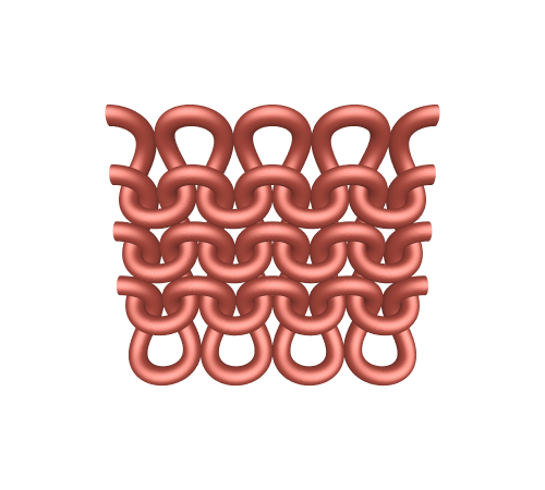
1. Yarn curves¶
#K. Crane's yarn curve rotated π/2 about y-axis, then π/2 about x-axis
γ(t; a=1.5, h=4, d=1) = [d*cos(2t),   t+a*sin(2t),  h*cos(t)]
u = range(0, 8π, length=600)
v = range(0, 2π, length=100);

x, y, z = [getindex.(tube.(γ,  u, v'; radius=4/5), i) for i∈1:3]
fig1 = plot_data([surf(x, y, z .+ k*4.5) for k in 0:3])
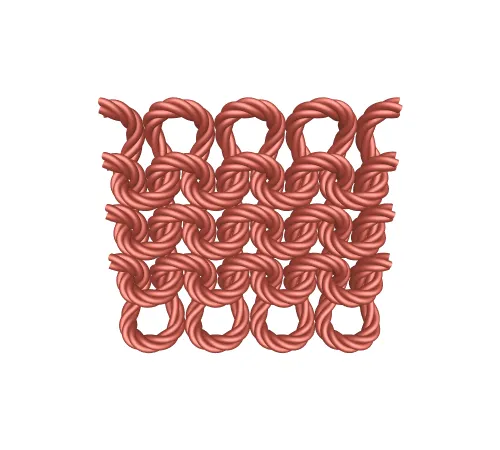
2. Twisted yarn fibers¶
γ(t; a=1.5, h=4, d=1)= [d*cos(2t),   t+a*sin(2t),  h*cos(t)] #curve
fcurves = [fiber_curve(γ; ω= 4,  Φ=k*π/2) for k ∈ 0:3];
u = range(0, 8π, length=600)
v = range(0, 2π, length=100);
fibers = GenericTrace{Dict{Symbol, Any}}[]
for fcurve  ∈ fcurves
    x, y, z = [getindex.(tube.(fcurve,  u, v'; radius=7/20), i)  for i∈ 1:3]
    push!(fibers, surf(x, y, z))
end
fig2 = plot_data(fibers)
Fiber curves for $\omega=2, 4, 6$:
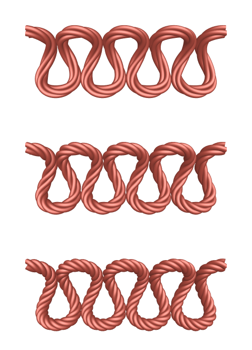
fibers = GenericTrace{Dict{Symbol, Any}}[]
for fcurve  ∈ fcurves
    x, y, z = [getindex.(tube.(fcurve,  u, v'; radius=7/20),i)  for i∈ 1:3]
    append!(fibers, [surf(x, y, z .+ j*4.5) for j∈0:3])#a fiber contains 4 twisted yarns(j=0:3)
end
fig3 = plot_data(fibers)