Classify "Quick, draw!" drawings
How to implement an image classifier in PyTorch?
- Data pipeline - DataSet, Data Augmentation
- Implementation - PyTorch Modules
- ConvNets - Convolution, learn Kernels, Pooling
"Can a neural network learn to recognize doodling?" - quickdraw.withgoogle.com

Import libraries
import torch
print("Torch version:", torch.__version__)

import torchvision
print("Torchvision version:", torchvision.__version__)

import numpy as np
print("Numpy version:", np.__version__)

import matplotlib
print("Matplotlib version:", matplotlib.__version__)

import PIL
print("PIL version:", PIL.__version__)

import IPython
print("IPython version:", IPython.__version__)
# Setup Matplotlib
%matplotlib inline
#%config InlineBackend.figure_format = 'retina' # If you have a retina screen
import matplotlib.pyplot as plt
A QuickDraw DataSet
More about PyTorch - Data Loading and Processing Tutorial by Sasank Chilamkurthy
- How to encapsulate a data set? - DataSet
- How to perform Data augmentation? - Transformation pipelines
Download Numpy bitmap files .npy - npy files from Google Cloud / GitHub repository
Possible classes: Airplanes - Cars - Cats - Ships

# If your are on mybinder.org, you can use this code to download the data
!mkdir -p data
!wget "https://storage.googleapis.com/quickdraw_dataset/full/numpy_bitmap/aircraft%20carrier.npy" -O "data/airplane.npy" -q --show-progress
!wget "https://storage.googleapis.com/quickdraw_dataset/full/numpy_bitmap/car.npy" -O "data/car.npy" -q --show-progress
!wget "https://storage.googleapis.com/quickdraw_dataset/full/numpy_bitmap/cat.npy" -O "data/cat.npy" -q --show-progress
!wget "https://storage.googleapis.com/quickdraw_dataset/full/numpy_bitmap/cruise%20ship.npy" -O "data/cruise ship.npy" -q --show-progress
import os

# Collect files
npy_files = [
    os.path.join('data', 'airplane.npy'),
    os.path.join('data', 'car.npy'),
    os.path.join('data', 'cat.npy'),
    os.path.join('data', 'cruise ship.npy'),
]
classes = ['plane', 'car', 'cat', 'ship']
from PIL import Image

# Create a class for our data set
class QuickDraw(torch.utils.data.Dataset):
    def __init__(self, npy_files, transform=None):
        # Open .npy files
        self.X_list = [np.load(f, mmap_mode='r') for f in npy_files]
        self.lengths = [len(X) for X in self.X_list]

        # Transformation pipeline
        self.transform = transform

    def __len__(self):
        return sum(self.lengths)

    def get_pixels(self, idx):
        for label, (X, l) in enumerate(zip(self.X_list, self.lengths)):
            if idx < l:
                return X[idx], label
            idx -= l

    def __getitem__(self, idx):
        # Get image
        img, label = self.get_pixels(idx)
        pil_img = Image.fromarray(255 - img.reshape(28, 28)) # White background

        # Transform image
        processed_img = self.transform(pil_img) if self.transform else pil_img

        return processed_img, label

# Create the data set
dataset = QuickDraw(npy_files)
print('Size:', len(dataset))
dataset[0][0]
from torchvision import transforms

# Data augmentation
t = transforms.Compose([
    transforms.RandomAffine(degrees=25, translate=(0.1, 0.1), shear=5, fillcolor=255),
    transforms.RandomHorizontalFlip()
])

dataset = QuickDraw(npy_files, t)
print('Size:', len(dataset))
# Get first image
dataset[0][0]
Data loaders
The next steps of the Data Pipeline in PyTorch
- Data Samplers - Train, Validation samplers
- Data Loaders - Combine DataSet, DataSampler
from torch.utils.data.sampler import SubsetRandomSampler

# Define train/validation sets
idx = np.arange(len(dataset)) # idx: 0 .. (n_images - 1)
np.random.shuffle(idx) # shuffle

# Create train/validation samplers
valid_size = 500
train_sampler = SubsetRandomSampler(idx[:-valid_size])
valid_sampler = SubsetRandomSampler(idx[-valid_size:])

print('Train set:', len(train_sampler))
print('Validation set:', len(valid_sampler))
from torch.utils.data import DataLoader

# Data augmentation for the "training" set
train_t = transforms.Compose([
    transforms.RandomHorizontalFlip(),
    transforms.ToTensor(),
    transforms.Normalize((0.829,), (0.326,)) # Computed on the train set
])
valid_t = transforms.Compose([
    transforms.ToTensor(),
    transforms.Normalize((0.829,), (0.326,))
])

# Create DataSets
train_set = QuickDraw(npy_files, train_t)
valid_set = QuickDraw(npy_files, valid_t)

# Create DataLoaders
train_loader = DataLoader(train_set, batch_size=64, sampler=train_sampler)
valid_loader = DataLoader(valid_set, batch_size=64, sampler=valid_sampler)

# Plot sample images
images, labels = next(iter(train_loader))
print('Labels:', labels)

grid = torchvision.utils.make_grid(images, normalize=True)
plt.imshow(grid.numpy().transpose((1, 2, 0)))
plt.show()
Fully-connected Network
What are the different ways to define a Network in PyTorch?
- Sequential Class - Add layers from nn module
- Create a NN Module - Subclass of torch.nn.Module or others, ex. torch.nn.Sequential
PyTorch nn.Module - link to the documentation
torch.nn.Module- Base class for all neural network modules. Your models should also subclass this class. Modules can also contain other Modules, allowing to nest them in a tree structure. You can assign the submodules as regular attributes: Submodules assigned in this way will be registered, and will have their parameters converted too when you call .cuda(), etc.
# Create a FullyConnected "Sequential" Module
class FullyConnected(torch.nn.Sequential):
    def __init__(self, n_in, n_out, h_units=[]):
        # Initialize module
        super().__init__()

        # Save network parameters
        self.n_inputs = n_in
        self.n_outputs = n_out
        self.h_units = h_units

        # Add hidden layers
        n_hidden = len(h_units)
        for i in range(n_hidden):
            # Input/output sizes
            hidden_in = n_in if i == 0 else h_units[i-1]
            hidden_out = h_units[i]

            # Add layer and activation
            self.add_module('hidden_{}'.format(i+1), torch.nn.Linear(hidden_in, hidden_out))
            self.add_module('relu_{}'.format(i+1), torch.nn.ReLU())

        # Add output layer
        output_in = n_in if n_hidden == 0 else hidden_out
        self.add_module('output', torch.nn.Linear(output_in, n_out))

    def forward(self, img):
        flat_img = img.view(-1, self.n_inputs)
        return super().forward(flat_img)

# Test
model = FullyConnected(28*28, len(classes))
model
Task - How to access Model Parameters?
- Plot weights from the first layer
# Visualize 1st layer of a FC network
def plot_weights(weights_fc1, axis):
    # Shape of weights matrix
    n_out, n_in = weights_fc1.shape

    # Create a grid
    n_cells = min(16, n_out)
    grid = torchvision.utils.make_grid(
        weights_fc1[:n_cells].view(n_cells, 1, 28, 28),
        nrow=4, normalize=True
    )

    # Plot it
    axis.imshow(grid.numpy().transpose((1, 2, 0)),)

# TODO - Plot weights from "model" 1st layer
Train the Model
Tasks - What is a good Network Architecture?
- 2-layer FC network - Best accuracy?
- Deeper network - Can you improve results?
from collections import defaultdict

# Create model
model = FullyConnected(28*28, len(classes))

# Criterion and optimizer for "training"
criterion = torch.nn.CrossEntropyLoss()
optimizer = torch.optim.SGD(model.parameters(), lr=0.01, weight_decay=1)

# Backprop step
def compute_loss(output, target):
    y_tensor = torch.LongTensor(target)
    y_variable = torch.autograd.Variable(y_tensor)
    return criterion(output, y_variable)

def backpropagation(output, target):
    optimizer.zero_grad() # Clear the gradients
    loss = compute_loss(output, target) # Compute loss
    loss.backward() # Backpropagation
    optimizer.step() # Let the optimizer adjust our model
    return loss.data

# Helper function
def get_accuracy(output, y):
    predictions = torch.argmax(output, dim=1) # Max activation
    is_correct = np.equal(predictions, y)
    return is_correct.numpy().mean()

# Create a figure to visualize the results
fig, (ax1, ax2, ax3) = plt.subplots(nrows=1, ncols=3, figsize=(12, 3))

try:
    # Collect loss / accuracy values
    stats = defaultdict(list)
    t = 0 # Number of samples seen
    print_step = 200 # Refresh rate

    for epoch in range(1, 10**5):
        # Train by small batches of data
        for batch, (batch_X, batch_y) in enumerate(train_loader, 1):
            # Forward pass & backpropagation
            output = model(batch_X)
            loss = backpropagation(output, batch_y)

            # Log "train" stats
            stats['train_loss'].append(loss)
            stats['train_acc'].append(get_accuracy(output, batch_y))
            stats['train_t'].append(t)

            if t%print_step == 0:
                # Log "validation" stats
                loss_vals, acc_vals = [], []
                for X, y in valid_loader:
                    output = model(X)
                    loss_vals.append(compute_loss(output, y).data)
                    acc_vals.append(get_accuracy(output, y))

                stats['val_loss'].append(np.mean(loss_vals))
                stats['val_acc'].append(np.mean(acc_vals))
                stats['val_t'].append(t)

                # Plot what the network learned
                ax1.cla()
                ax1.set_title('Epoch {}, batch {:,}'.format(epoch, batch))
                plot_weights(model[0].weight.data, ax1)
                ax2.cla()
                ax2.set_title('Loss, val: {:.3f}'.format(np.mean(stats['val_loss'][-10:])))
                ax2.plot(stats['train_t'], stats['train_loss'], label='train')
                ax2.plot(stats['val_t'], stats['val_loss'], label='valid')
                ax2.legend()
                ax3.cla()
                ax3.set_title('Accuracy, val: {:.3f}'.format(np.mean(stats['val_acc'][-10:])))
                ax3.plot(stats['train_t'], stats['train_acc'], label='train')
                ax3.plot(stats['val_t'], stats['val_acc'], label='valid')
                ax3.set_ylim(0, 1)
                ax3.legend()

                # Jupyter trick
                IPython.display.clear_output(wait=True)
                IPython.display.display(fig)

            # Update t
            t += train_loader.batch_size

except KeyboardInterrupt:
    # Clear output
    IPython.display.clear_output()
Convolutional Network
"Make some assumptions about the inputs to make learning more efficient" - Andrej Karpathy Lecture
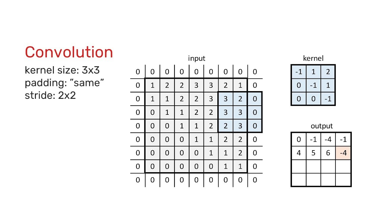
Convolutional Layers Parameters
- Kernel Size - Size of our "Feature Detectors"
- Output depth - Number of kernels
- Stride - How they move
- Padding - Add "borders" to the inputs
Pooling Parameters
- Pooling function - Maximum, Average
- Size and Stride - Downsampling ex. size=2 and stride=2
Implementation - Inspired by AlexNet PyTorch Code
from collections import namedtuple

# Create a Pooling Named Tuple
PoolParams = namedtuple('PoolParams', ['size', 'stride'])
sample_poolparams = PoolParams(size=2, stride=2)

# Create a ConvParams Named Tuple
ConvParams = namedtuple('ConvParams', ['size', 'n_kernels', 'stride', 'pooling'])
sample_convparams = ConvParams(size=16, n_kernels=5, stride=2, pooling=None)

# Create an InputShape Named Tuple
InputShape = namedtuple('InputShape', ['channels', 'height', 'width'])
images_shape = InputShape(channels=1, height=28, width=28)

# Create a ConvNet Module
class ConvNet(torch.nn.Module):
    def __init__(self, layers_params, input_shape):
        # Initialize module
        super().__init__()

        # "Feature extraction" part
        self.features = torch.nn.Sequential()
        for layer_no, (size, n_kernels, stride, pooling) in enumerate(layers_params, 1):
            # Input depth
            depth_in = input_shape.channels if layer_no == 1 else layers_params[layer_no-2].n_kernels

            # Convolutional Layer
            self.features.add_module(
                'conv2d_{}'.format(layer_no),
                torch.nn.Conv2d(depth_in, n_kernels, size, stride)
            )
            self.features.add_module('relu_{}'.format(layer_no), torch.nn.ReLU())

            # Max-pooling layer
            if pooling is not None:
                self.features.add_module('maxpool_{}'.format(layer_no), torch.nn.MaxPool2d(pooling.size, pooling.stride))

        # Compute the number of features extracted
        sample_input = torch.zeros(1, input_shape.channels, input_shape.height, input_shape.width)
        _, depth_out, height_out, width_out = self.features(sample_input).shape
        self.n_features = depth_out*height_out*width_out

        # "Classifier" part
        self.classifier = torch.nn.Sequential(
            torch.nn.Linear(self.n_features, 10)
        )

    def forward(self, img):
        # Extract features
        img_features = self.features(img)
        flat_features = img_features.view(-1, self.n_features)

        # Classify image
        return self.classifier(flat_features)

# Create toy model
model = ConvNet([
    ConvParams(size=5, n_kernels=16, stride=2, pooling=PoolParams(size=2, stride=2)),
    ConvParams(size=3, n_kernels=32, stride=1, pooling=PoolParams(size=2, stride=2)),
], images_shape)
model
# Try forward pass
print('Sample input:', images.shape)
print('Sample output:', model(images).shape)
How to access Model Parameters?
# Visualize kernels from the 1st Convolutional Layer
def plot_kernels(model, axis):
    # Weights
    kernel_weights = model.features.conv2d_1.weight.data
    n_kernels, in_depth, height, width = kernel_weights.shape

    # Create a grid
    n_cells = min(16, n_kernels)
    grid = torchvision.utils.make_grid(
        kernel_weights[:n_cells, 0].view(n_cells, in_depth, height, width),
        nrow=4, normalize=True, padding=1
    )

    # Plot it
    axis.imshow(grid.numpy().transpose((1, 2, 0)),)

fig = plt.figure(figsize=(3, 3))
plot_kernels(model, fig.gca())
Tasks - Convolutional Nets
- Train model - Adapt "training" code from above for ConvNets
- Model Architecture - Play with the different parameters, best accuracy?
# TODO - Train ConvNet here
Small challenges
- Print the number of parameters in each layer
- Pass a few images and print the outputs shapes
- Plot the "activation maps" for a sample input
Additional resources
Nice visualizations
- Deep Visualization Toolbox - Presentation on YouTube / GitHub repository
- Feature Visualization - distill.pub article
- The Building Blocks of Interpretability - distill.pub article
To go deeper
- ImageNet Classification with Deep Convolutional Neural Networks - Slides