In [ ]:

%load_ext autoreload
%autoreload 2

%matplotlib inline

In [ ]:

#export
from exp.nb_06 import *

ConvNet¶

Let's get the data and training interface from where we left in the last notebook.

Jump_to lesson 10 video

In [ ]:

x_train,y_train,x_valid,y_valid = get_data()

x_train,x_valid = normalize_to(x_train,x_valid)
train_ds,valid_ds = Dataset(x_train, y_train),Dataset(x_valid, y_valid)

nh,bs = 50,512
c = y_train.max().item()+1
loss_func = F.cross_entropy

data = DataBunch(*get_dls(train_ds, valid_ds, bs), c)

In [ ]:

mnist_view = view_tfm(1,28,28)
cbfs = [Recorder,
        partial(AvgStatsCallback,accuracy),
        CudaCallback,
        partial(BatchTransformXCallback, mnist_view)]

In [ ]:

nfs = [8,16,32,64,64]

In [ ]:

learn,run = get_learn_run(nfs, data, 0.4, conv_layer, cbs=cbfs)

In [ ]:

%time run.fit(2, learn)

train: [1.024234921875, tensor(0.6730, device='cuda:0')]
valid: [0.2444910400390625, tensor(0.9262, device='cuda:0')]
train: [0.162599970703125, tensor(0.9502, device='cuda:0')]
valid: [0.10074585571289063, tensor(0.9698, device='cuda:0')]
CPU times: user 3.78 s, sys: 1.61 s, total: 5.39 s
Wall time: 6.37 s

Batchnorm¶

Custom¶

Let's start by building our own BatchNorm layer from scratch.

Jump_to lesson 10 video

In [ ]:

class BatchNorm(nn.Module):
    def __init__(self, nf, mom=0.1, eps=1e-5):
        super().__init__()
        # NB: pytorch bn mom is opposite of what you'd expect
        self.mom,self.eps = mom,eps
        self.mults = nn.Parameter(torch.ones (nf,1,1))
        self.adds  = nn.Parameter(torch.zeros(nf,1,1))
        self.register_buffer('vars',  torch.ones(1,nf,1,1))
        self.register_buffer('means', torch.zeros(1,nf,1,1))

    def update_stats(self, x):
        m = x.mean((0,2,3), keepdim=True)
        v = x.var ((0,2,3), keepdim=True)
        self.means.lerp_(m, self.mom)
        self.vars.lerp_ (v, self.mom)
        return m,v
        
    def forward(self, x):
        if self.training:
            with torch.no_grad(): m,v = self.update_stats(x)
        else: m,v = self.means,self.vars
        x = (x-m) / (v+self.eps).sqrt()
        return x*self.mults + self.adds

In [ ]:

def conv_layer(ni, nf, ks=3, stride=2, bn=True, **kwargs):
    # No bias needed if using bn
    layers = [nn.Conv2d(ni, nf, ks, padding=ks//2, stride=stride, bias=not bn),
              GeneralRelu(**kwargs)]
    if bn: layers.append(BatchNorm(nf))
    return nn.Sequential(*layers)

In [ ]:

#export
def init_cnn_(m, f):
    if isinstance(m, nn.Conv2d):
        f(m.weight, a=0.1)
        if getattr(m, 'bias', None) is not None: m.bias.data.zero_()
    for l in m.children(): init_cnn_(l, f)

def init_cnn(m, uniform=False):
    f = init.kaiming_uniform_ if uniform else init.kaiming_normal_
    init_cnn_(m, f)

def get_learn_run(nfs, data, lr, layer, cbs=None, opt_func=None, uniform=False, **kwargs):
    model = get_cnn_model(data, nfs, layer, **kwargs)
    init_cnn(model, uniform=uniform)
    return get_runner(model, data, lr=lr, cbs=cbs, opt_func=opt_func)

We can then use it in training and see how it helps keep the activations means to 0 and the std to 1.

In [ ]:

learn,run = get_learn_run(nfs, data, 0.9, conv_layer, cbs=cbfs)

In [ ]:

with Hooks(learn.model, append_stats) as hooks:
    run.fit(1, learn)
    fig,(ax0,ax1) = plt.subplots(1,2, figsize=(10,4))
    for h in hooks[:-1]:
        ms,ss = h.stats
        ax0.plot(ms[:10])
        ax1.plot(ss[:10])
        h.remove()
    plt.legend(range(6));
    
    fig,(ax0,ax1) = plt.subplots(1,2, figsize=(10,4))
    for h in hooks[:-1]:
        ms,ss = h.stats
        ax0.plot(ms)
        ax1.plot(ss)

train: [0.26532763671875, tensor(0.9189, device='cuda:0')]
valid: [0.16395225830078125, tensor(0.9520, device='cuda:0')]

In [ ]:

learn,run = get_learn_run(nfs, data, 1.0, conv_layer, cbs=cbfs)

In [ ]:

%time run.fit(3, learn)

train: [0.27833810546875, tensor(0.9105, device='cuda:0')]
valid: [0.1912491943359375, tensor(0.9386, device='cuda:0')]
train: [0.08977265625, tensor(0.9713, device='cuda:0')]
valid: [0.09156090698242188, tensor(0.9716, device='cuda:0')]
train: [0.06145498046875, tensor(0.9810, device='cuda:0')]
valid: [0.09970919799804688, tensor(0.9707, device='cuda:0')]
CPU times: user 3.71 s, sys: 584 ms, total: 4.29 s
Wall time: 4.29 s

Builtin batchnorm¶

Jump_to lesson 10 video

In [ ]:

#export
def conv_layer(ni, nf, ks=3, stride=2, bn=True, **kwargs):
    layers = [nn.Conv2d(ni, nf, ks, padding=ks//2, stride=stride, bias=not bn),
              GeneralRelu(**kwargs)]
    if bn: layers.append(nn.BatchNorm2d(nf, eps=1e-5, momentum=0.1))
    return nn.Sequential(*layers)

In [ ]:

learn,run = get_learn_run(nfs, data, 1., conv_layer, cbs=cbfs)

In [ ]:

%time run.fit(3, learn)

train: [0.27115255859375, tensor(0.9206, device='cuda:0')]
valid: [0.1547997314453125, tensor(0.9496, device='cuda:0')]
train: [0.07861462890625, tensor(0.9755, device='cuda:0')]
valid: [0.07472044067382813, tensor(0.9776, device='cuda:0')]
train: [0.0570835498046875, tensor(0.9818, device='cuda:0')]
valid: [0.0673232666015625, tensor(0.9813, device='cuda:0')]
CPU times: user 3.37 s, sys: 747 ms, total: 4.12 s
Wall time: 4.12 s

With scheduler¶

Now let's add the usual warm-up/annealing.

In [ ]:

sched = combine_scheds([0.3, 0.7], [sched_lin(0.6, 2.), sched_lin(2., 0.1)]) 

In [ ]:

learn,run = get_learn_run(nfs, data, 0.9, conv_layer, cbs=cbfs
                          +[partial(ParamScheduler,'lr', sched)])

In [ ]:

run.fit(8, learn)

train: [0.2881914453125, tensor(0.9116, device='cuda:0')]
valid: [0.5269224609375, tensor(0.8394, device='cuda:0')]
train: [0.153792421875, tensor(0.9551, device='cuda:0')]
valid: [0.462953662109375, tensor(0.8514, device='cuda:0')]
train: [0.087637158203125, tensor(0.9736, device='cuda:0')]
valid: [0.07029829711914062, tensor(0.9788, device='cuda:0')]
train: [0.049282421875, tensor(0.9853, device='cuda:0')]
valid: [0.08710025024414063, tensor(0.9740, device='cuda:0')]
train: [0.0356986328125, tensor(0.9888, device='cuda:0')]
valid: [0.07853966674804687, tensor(0.9773, device='cuda:0')]
train: [0.0268300439453125, tensor(0.9918, device='cuda:0')]
valid: [0.04807376098632812, tensor(0.9870, device='cuda:0')]
train: [0.0219412109375, tensor(0.9939, device='cuda:0')]
valid: [0.04363873901367187, tensor(0.9882, device='cuda:0')]
train: [0.018501048583984374, tensor(0.9951, device='cuda:0')]
valid: [0.04355916137695313, tensor(0.9877, device='cuda:0')]

More norms¶

Layer norm¶

From the paper: "batch normalization cannot be applied to online learning tasks or to extremely large distributed models where the minibatches have to be small".

General equation for a norm layer with learnable affine:

$$y = \frac{x - \mathrm{E}[x]}{ \sqrt{\mathrm{Var}[x] + \epsilon}} * \gamma + \beta$$

The difference with BatchNorm is

we don't keep a moving average
we don't average over the batches dimension but over the hidden dimension, so it's independent of the batch size

Jump_to lesson 10 video

In [ ]:

class LayerNorm(nn.Module):
    __constants__ = ['eps']
    def __init__(self, eps=1e-5):
        super().__init__()
        self.eps = eps
        self.mult = nn.Parameter(tensor(1.))
        self.add  = nn.Parameter(tensor(0.))

    def forward(self, x):
        m = x.mean((1,2,3), keepdim=True)
        v = x.var ((1,2,3), keepdim=True)
        x = (x-m) / ((v+self.eps).sqrt())
        return x*self.mult + self.add

In [ ]:

def conv_ln(ni, nf, ks=3, stride=2, bn=True, **kwargs):
    layers = [nn.Conv2d(ni, nf, ks, padding=ks//2, stride=stride, bias=True),
              GeneralRelu(**kwargs)]
    if bn: layers.append(LayerNorm())
    return nn.Sequential(*layers)

In [ ]:

learn,run = get_learn_run(nfs, data, 0.8, conv_ln, cbs=cbfs)

In [ ]:

%time run.fit(3, learn)

train: [nan, tensor(0.1321, device='cuda:0')]
valid: [nan, tensor(0.0991, device='cuda:0')]
train: [nan, tensor(0.0986, device='cuda:0')]
valid: [nan, tensor(0.0991, device='cuda:0')]
train: [nan, tensor(0.0986, device='cuda:0')]
valid: [nan, tensor(0.0991, device='cuda:0')]
CPU times: user 4.56 s, sys: 862 ms, total: 5.42 s
Wall time: 5.42 s

Thought experiment: can this distinguish foggy days from sunny days (assuming you're using it before the first conv)?

Instance norm¶

From the paper:

The key difference between contrast and batch normalization is that the latter applies the normalization to a whole batch of images instead for single ones:

\begin{equation}\label{eq:bnorm} y_{tijk} = \frac{x_{tijk} - \mu_{i}}{\sqrt{\sigma_i^2 + \epsilon}}, \quad \mu_i = \frac{1}{HWT}\sum_{t=1}^T\sum_{l=1}^W \sum_{m=1}^H x_{tilm}, \quad \sigma_i^2 = \frac{1}{HWT}\sum_{t=1}^T\sum_{l=1}^W \sum_{m=1}^H (x_{tilm} - mu_i)^2. \end{equation}

In order to combine the effects of instance-specific normalization and batch normalization, we propose to replace the latter by the instance normalization (also known as contrast normalization) layer:

\begin{equation}\label{eq:inorm} y_{tijk} = \frac{x_{tijk} - \mu_{ti}}{\sqrt{\sigma_{ti}^2 + \epsilon}}, \quad \mu_{ti} = \frac{1}{HW}\sum_{l=1}^W \sum_{m=1}^H x_{tilm}, \quad \sigma_{ti}^2 = \frac{1}{HW}\sum_{l=1}^W \sum_{m=1}^H (x_{tilm} - mu_{ti})^2. \end{equation}

Jump_to lesson 10 video

In [ ]:

class InstanceNorm(nn.Module):
    __constants__ = ['eps']
    def __init__(self, nf, eps=1e-0):
        super().__init__()
        self.eps = eps
        self.mults = nn.Parameter(torch.ones (nf,1,1))
        self.adds  = nn.Parameter(torch.zeros(nf,1,1))

    def forward(self, x):
        m = x.mean((2,3), keepdim=True)
        v = x.var ((2,3), keepdim=True)
        res = (x-m) / ((v+self.eps).sqrt())
        return res*self.mults + self.adds

In [ ]:

def conv_in(ni, nf, ks=3, stride=2, bn=True, **kwargs):
    layers = [nn.Conv2d(ni, nf, ks, padding=ks//2, stride=stride, bias=True),
              GeneralRelu(**kwargs)]
    if bn: layers.append(InstanceNorm(nf))
    return nn.Sequential(*layers)

In [ ]:

learn,run = get_learn_run(nfs, data, 0.1, conv_in, cbs=cbfs)

In [ ]:

%time run.fit(3, learn)

train: [nan, tensor(0.0986, device='cuda:0')]
valid: [nan, tensor(0.0991, device='cuda:0')]
train: [nan, tensor(0.0986, device='cuda:0')]
valid: [nan, tensor(0.0991, device='cuda:0')]
train: [nan, tensor(0.0986, device='cuda:0')]
valid: [nan, tensor(0.0991, device='cuda:0')]
CPU times: user 4.46 s, sys: 718 ms, total: 5.18 s
Wall time: 5.18 s

Question: why can't this classify anything?

Lost in all those norms? The authors from the group norm paper have you covered:

Various norms

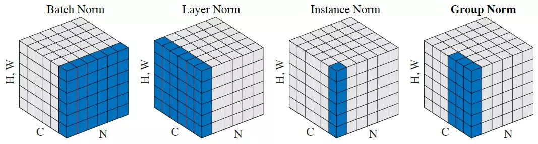
Group norm¶

Jump_to lesson 10 video

From the PyTorch docs:

GroupNorm(num_groups, num_channels, eps=1e-5, affine=True)

The input channels are separated into num_groups groups, each containing num_channels / num_groups channels. The mean and standard-deviation are calculated separately over the each group. $\gamma$ and $\beta$ are learnable per-channel affine transform parameter vectorss of size num_channels if affine is True.

This layer uses statistics computed from input data in both training and evaluation modes.

Args:

num_groups (int): number of groups to separate the channels into
num_channels (int): number of channels expected in input
eps: a value added to the denominator for numerical stability. Default: 1e-5
affine: a boolean value that when set to True, this module has learnable per-channel affine parameters initialized to ones (for weights) and zeros (for biases). Default: True.

Shape:

Input: (N, num_channels, *)
Output: (N, num_channels, *) (same shape as input)

Examples::

>>> input = torch.randn(20, 6, 10, 10)
>>> # Separate 6 channels into 3 groups
>>> m = nn.GroupNorm(3, 6)
>>> # Separate 6 channels into 6 groups (equivalent with InstanceNorm)
>>> m = nn.GroupNorm(6, 6)
>>> # Put all 6 channels into a single group (equivalent with LayerNorm)
>>> m = nn.GroupNorm(1, 6)
>>> # Activating the module
>>> output = m(input)

Fix small batch sizes¶

What's the problem?¶

When we compute the statistics (mean and std) for a BatchNorm Layer on a small batch, it is possible that we get a standard deviation very close to 0. because there aren't many samples (the variance of one thing is 0. since it's equal to its mean).

Jump_to lesson 10 video

In [ ]:

data = DataBunch(*get_dls(train_ds, valid_ds, 2), c)

In [ ]:

def conv_layer(ni, nf, ks=3, stride=2, bn=True, **kwargs):
    layers = [nn.Conv2d(ni, nf, ks, padding=ks//2, stride=stride, bias=not bn),
              GeneralRelu(**kwargs)]
    if bn: layers.append(nn.BatchNorm2d(nf, eps=1e-5, momentum=0.1))
    return nn.Sequential(*layers)

In [ ]:

learn,run = get_learn_run(nfs, data, 0.4, conv_layer, cbs=cbfs)

In [ ]:

%time run.fit(1, learn)

train: [2.35619296875, tensor(0.1649, device='cuda:0')]
valid: [2867.7198, tensor(0.2604, device='cuda:0')]
CPU times: user 1min 32s, sys: 835 ms, total: 1min 33s
Wall time: 1min 33s

Running Batch Norm¶

To solve this problem we introduce a Running BatchNorm that uses smoother running mean and variance for the mean and std.

Jump_to lesson 10 video

In [ ]:

class RunningBatchNorm(nn.Module):
    def __init__(self, nf, mom=0.1, eps=1e-5):
        super().__init__()
        self.mom,self.eps = mom,eps
        self.mults = nn.Parameter(torch.ones (nf,1,1))
        self.adds = nn.Parameter(torch.zeros(nf,1,1))
        self.register_buffer('sums', torch.zeros(1,nf,1,1))
        self.register_buffer('sqrs', torch.zeros(1,nf,1,1))
        self.register_buffer('batch', tensor(0.))
        self.register_buffer('count', tensor(0.))
        self.register_buffer('step', tensor(0.))
        self.register_buffer('dbias', tensor(0.))

    def update_stats(self, x):
        bs,nc,*_ = x.shape
        self.sums.detach_()
        self.sqrs.detach_()
        dims = (0,2,3)
        s = x.sum(dims, keepdim=True)
        ss = (x*x).sum(dims, keepdim=True)
        c = self.count.new_tensor(x.numel()/nc)
        mom1 = 1 - (1-self.mom)/math.sqrt(bs-1)
        self.mom1 = self.dbias.new_tensor(mom1)
        self.sums.lerp_(s, self.mom1)
        self.sqrs.lerp_(ss, self.mom1)
        self.count.lerp_(c, self.mom1)
        self.dbias = self.dbias*(1-self.mom1) + self.mom1
        self.batch += bs
        self.step += 1

    def forward(self, x):
        if self.training: self.update_stats(x)
        sums = self.sums
        sqrs = self.sqrs
        c = self.count
        if self.step<100:
            sums = sums / self.dbias
            sqrs = sqrs / self.dbias
            c    = c    / self.dbias
        means = sums/c
        vars = (sqrs/c).sub_(means*means)
        if bool(self.batch < 20): vars.clamp_min_(0.01)
        x = (x-means).div_((vars.add_(self.eps)).sqrt())
        return x.mul_(self.mults).add_(self.adds)

In [ ]:

def conv_rbn(ni, nf, ks=3, stride=2, bn=True, **kwargs):
    layers = [nn.Conv2d(ni, nf, ks, padding=ks//2, stride=stride, bias=not bn),
              GeneralRelu(**kwargs)]
    if bn: layers.append(RunningBatchNorm(nf))
    return nn.Sequential(*layers)

In [ ]:

learn,run = get_learn_run(nfs, data, 0.4, conv_rbn, cbs=cbfs)

In [ ]:

%time run.fit(1, learn)

train: [0.157932021484375, tensor(0.9511, device='cuda:0')]
valid: [0.0986408935546875, tensor(0.9730, device='cuda:0')]
CPU times: user 16.5 s, sys: 1.57 s, total: 18.1 s
Wall time: 18.1 s

This solves the small batch size issue!

What can we do in a single epoch?¶

Now let's see with a decent batch size what result we can get.

Jump_to lesson 10 video

In [ ]:

data = DataBunch(*get_dls(train_ds, valid_ds, 32), c)

In [ ]:

learn,run = get_learn_run(nfs, data, 0.9, conv_rbn, cbs=cbfs
                          +[partial(ParamScheduler,'lr', sched_lin(1., 0.2))])

In [ ]:

%time run.fit(1, learn)

train: [0.1573110546875, tensor(0.9521, device='cuda:0')]
valid: [0.09242745971679688, tensor(0.9818, device='cuda:0')]
CPU times: user 16.6 s, sys: 1.52 s, total: 18.1 s
Wall time: 18.2 s

Export¶

In [ ]:

nb_auto_export()

In [ ]: