JuliaとJupyterのすすめ
- Author: 黒木 玄
- Date: 2019-03-16~2019-06-30
- Repository: https://github.com/genkuroki/msfd28
注意: 筆者は「ライトユーザー」なので深い話はできない.
このファイルは以下の研究会のために準備された:
- 数学ソフトウェアとフリードキュメント XXVIII
- 2019年3月16日(土) 13:00–18:00
- 東京工業大学 大岡山キャンパス 本館1階H116講義室
この文書は以下の場所で閲覧できる:
私によるJulia+Jupyterの環境構築の最近の記録については次のメモを参照せよ:
目次
- 1 Jupyterノートブック
- 2 Julia言語
- 3 グルー言語としてのJulia
- 4 ギャラリー
- 5 ツイッターで紹介したJuliaの使い方のリスト
- 6 ツイッターで教えてもらったJuliaの使い方
- 7 おまけ
print("using Plots ->")
@time using Plots
gr(legend=false); ENV["PLOTS_TEST"] = "true"
print("\nplot(sin) ->")
@time plot(sin, size=(300, 160)) |> display # コンパイル
print("\nusing PyPlot ->")
@time using PyPlot: PyPlot, plt
print("\nusing DifferentialEquations ->")
@time using DifferentialEquations
using Base64
using Combinatorics
using Distributed
using Distributions
using Libdl
using LinearAlgebra
using Optim
using Primes
using ProgressMeter
using Random: seed!
using RCall
using SpecialFunctions
using Statistics
using SymPy: SymPy, sympy, Sym, @vars, @syms, simplify, oo, PI
ldisp(x...) = display("text/html", raw"$$" * prod(x) * raw"$$")
showimg(mime, fn) = open(fn) do f
base64 = base64encode(f)
display("text/html", """<img src="data:$mime;base64,$base64">""")
end
using Plots -> 6.497952 seconds (10.35 M allocations: 547.218 MiB, 5.71% gc time)
plot(sin) -> 25.666761 seconds (56.63 M allocations: 2.761 GiB, 6.50% gc time) using PyPlot -> 7.997156 seconds (14.13 M allocations: 696.137 MiB, 5.28% gc time) using DifferentialEquations -> 13.710626 seconds (35.83 M allocations: 2.302 GiB, 8.87% gc time) R version 3.5.3 (2019-03-11) -- "Great Truth" Copyright (C) 2019 The R Foundation for Statistical Computing Platform: x86_64-w64-mingw32/x64 (64-bit) R is free software and comes with ABSOLUTELY NO WARRANTY. You are welcome to redistribute it under certain conditions. Type 'license()' or 'licence()' for distribution details. R is a collaborative project with many contributors. Type 'contributors()' for more information and 'citation()' on how to cite R or R packages in publications. Type 'demo()' for some demos, 'help()' for on-line help, or 'help.start()' for an HTML browser interface to help. Type 'q()' to quit R.
showimg (generic function with 1 method)
パッケージの読み込みと最初の実行時のコンパイルにそれなりに時間が採られることに注意.
Jupyter notebook では最初のセルで最初のコンパイルが実行されるようにしておき, そのセルを実行してから, プログラムのコードの入力を始めると時間の節約になる.
Jupyterノートブック
このファイルはJupyterノートブックの実例になっている.
JupyterではJulia, Python, R, Rubyなどのプログラミング言語のノートブックを作れる.
ノートブックにはブラウザ経由でアクセスする.
ノートブックには以下をまとめることができる:
- プログラムのコード
- その実行結果(グラフのプロットを含む)
- 整形された数式を含む説明(markdown)
Jupterノートブックの表示にGitHubなどが対応している(nbviewerが非常に便利).
試行錯誤に向いている.
数百行程度のプログラミングにはこれで十分.
NbextensionsのGist-itを使えば, ワンタッチでノートブックをGitHub Gistに保存してバージョン管理できる.
NbextensionsのRISEを使えば, Jupyterノートブックでプレゼン可能.
JupyterはPythonのライブラリの1つ.
Anacondaを入れればJupyterも使えるようになっている.
追記(2019-05-26): Free Wolfram Engine が公開された. それとJupyterを組み合わせると「無料でMathematicaを使用」のような状態になる(実際にはJupyter側の対応が未成熟なので制限がある). 詳しくは
を参照して欲しい.
追記(2019-06-30): Jupyterという名前の由来については
を参照せよ(以下に画像として引用).
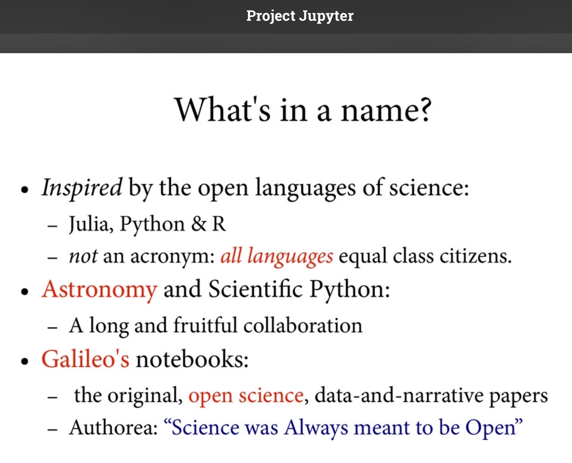
このように, Jupyter という名前は open languages of science である Julia, Python, R に着想を得ているが, それらの先頭部分を繋げたものではないと書かれており, すべてのプログラミング言語 を平等に扱うことが宣言されている. だから, Jupyterを一部のプログラミング言語(特にPython)専用の環境であるかのような印象を広めることは, Jupyterの作者たちの意向に反している. さらに open science を強調していることにも注目せよ.

整形された数式を含む説明の例
パラメーター $w$ 付きの $y$ に関する確率密度函数 $p(y|w)$ と事前分布と呼ばれる $w$ に関する確率密度函数 $\varphi(w)$ とサンプル $Y_1,\ldots,Y_n$ から得られるベイズ推測法における予測分布 $p^*(y)$ は以下のように定義される:
$$ p^*(y) = \frac{Z(Y_1,\ldots,Y_n,y|\varphi)}{Z(Y_1,\ldots,Y_n|\varphi)} = Z(y|\psi). $$ここで
$$ \begin{aligned} & Z(y_1,\ldots,y_n|\varphi) = \int \prod_{k=1}^n p(Y_k|w)\cdot\varphi(w)\,dw, \\ & \psi(w) = \frac{\prod_{k=1}^n p(Y_k|w)\cdot\varphi(w)}{\int \prod_{k=1}^n p(Y_k|w)\cdot\varphi(w)\,dw}. \end{aligned} $$$Z(y_1,\ldots,y_n|\varphi)$ は分配函数と呼ばれ, $Z(Y_1,\ldots,Y_n|\varphi)$ は周辺尤度と呼ばれ, $\psi(w)$ は事後分布と呼ばれる.
Just-in-time でコンパイル
Julia言語では
函数を実行したときに,
与えられた引数の型情報を使って,
その函数をネイティブコードにコンパイルしてから実行する.
こういう仕組みなので高速に計算したいコードは函数の中に入れなければいけない.
最初の実行時にはコンパイルにも時間が取られることに注意.
以下は円周率のモンテカルロ計算で比較.
### 函数にせずに実行
@time begin
L = 10^7
c = 0
for i in 1:L
global c
c += ifelse(rand()^2+rand()^2 ≤ 1, 1, 0)
end
4c/L
end
1.418559 seconds (40.00 M allocations: 762.914 MiB, 10.46% gc time)
3.1410228
### 函数にして実行
function simpi(L=10^7)
c = 0
for i in 1:L
c += ifelse(rand()^2+rand()^2 ≤ 1, 1, 0)
end
4c/L
end
simpi(10^5) # simpi(::Int64)がコンパイルされる
@time simpi()
0.047364 seconds (36.00 k allocations: 1.967 MiB)
3.141308
実行コードを函数の中に入れるだけで数十倍計算が速くなった.
Julia言語では各函数が引数の型情報に基いて just-in-time でコンパイルされる.
gccとの比較
円周率のモンテカルロ計算(1億回)で比較.
versioninfo()
Julia Version 1.1.0 Commit 80516ca202 (2019-01-21 21:24 UTC) Platform Info: OS: Windows (x86_64-w64-mingw32) CPU: Intel(R) Core(TM) i7-4770HQ CPU @ 2.20GHz WORD_SIZE: 64 LIBM: libopenlibm LLVM: libLLVM-6.0.1 (ORCJIT, haswell) Environment: JULIA_CMDSTAN_HOME = C:\CmdStan JULIA_NUM_THREADS = 4 JULIA_PKGDIR = C:\JuliaPkg
run(`gcc --version`); # ほとんど使っていないのでバージョンが古い
gcc (Rev3, Built by MSYS2 project) 6.3.0 Copyright (C) 2016 Free Software Foundation, Inc. This is free software; see the source for copying conditions. There is NO warranty; not even for MERCHANTABILITY or FITNESS FOR A PARTICULAR PURPOSE.
### gcc
C_code= raw"""
#include <time.h>
#include <stdlib.h>
double simpi(unsigned long n){
double x,y;
srand((unsigned)time(NULL));
double R = (double) RAND_MAX;
unsigned long count = 0;
for(unsigned long j=0; j < n; j++){
x = ((double) rand())/R;
y = ((double) rand())/R;
if(x*x + y*y <= 1){
count++;
}
}
return ((double) 4.0)*((double) count)/((double) n);
}
"""
filename = tempname()
filenamedl = filename * "." * Libdl.dlext
open(`gcc -Wall -O3 -march=native -xc -shared -o $filenamedl -`, "w") do f
print(f, C_code)
end
## run(`ls -l $filenamedl`);
const simpi_gcc_rand_lib = filename
simpi_gcc_rand(n::Int64) = ccall((:simpi, simpi_gcc_rand_lib), Float64, (Int64,), n)
simpi_gcc_rand(10^5)
@time simpi_gcc_rand(10^8)
2.537506 seconds (1.94 k allocations: 116.293 KiB)
3.14153524
### Julia
@time simpi(10^8)
0.392231 seconds (6 allocations: 192 bytes)
3.14148068
gccの側が圧倒的に遅い. Juliaの方が計算が数倍速い.
これはgccのデフォルトの rand() が遅いから.
そもそもgccの rand() は擬似乱数の質の点でモンテカルロシミュレーションには向かない.
Julia言語は dSFMT(Double precision SIMD-oriented Fast Mersenne Twister) をデフォルトの擬似乱数発生器として使っている.
gccの側でもdSFMTを使えば, Julia言語より少し速くなる.
注意: MT19937 より dSFMT の方が擬似乱数の質も上でかつ擬似乱数の発生速度も約3倍程速い(検証用コード). この点に MT19937 (所謂メルセンヌツイスター)の使用者は注意した方がよい. ライブラリ選択に関するこの手の問題は無数にあるので, 私程度の知識と実力だと gcc を使った場合よりも Julia を使った場合の方が計算が速くなることが多い. Julia言語は信頼できてかつ高速なライブラリの寄せ集めにもなっている.
以下で円周率のモンテカルロ計算(10億回)で比較.
### gcc with dSFMT
## Download http://www.math.sci.hiroshima-u.ac.jp/~m-mat/MT/SFMT/dSFMT-src-2.2.3.tar.gz
##
## Extract
## dSFMT-src-2.2.3/dSFMT.h
## dSFMT-src-2.2.3/dSFMT.c
C_code= raw"""
#include <stdio.h>
#include <stdlib.h>
#include <time.h>
#define HAVE_SSE2
#define DSFMT_MEXP 521
#include "dSFMT-src-2.2.3/dSFMT.h"
#include "dSFMT-src-2.2.3/dSFMT.c"
double simpi(unsigned long n){
srand((unsigned)time(NULL));
dsfmt_t dsfmt;
dsfmt_init_gen_rand(&dsfmt, rand());
unsigned long count = 0;
double x,y;
for(unsigned long j = 0; j < n; j++){
x = dsfmt_genrand_close_open(&dsfmt);
y = dsfmt_genrand_close_open(&dsfmt);
if(x*x + y*y <= 1){
count++;
}
}
return ((double)4.0)*((double)count)/((double)n);
}
"""
filename = tempname()
filenamedl = filename * "." * Libdl.dlext
open(`gcc -Wall -O3 -march=native -xc -shared -o $filenamedl -`, "w") do f
print(f, C_code)
end
## run(`ls -l $filenamedl`);
const simpi_gcc_dSFMT_lib = filename
simpi_gcc_dSFMT(n::Int64) = ccall((:simpi, simpi_gcc_dSFMT_lib), Float64, (Int64,), n)
simpi_gcc_dSFMT(10^5)
@time simpi_gcc_dSFMT(10^9)
2.928520 seconds (1.41 k allocations: 84.691 KiB)
3.14162012
### Julia
@time simpi(10^9)
3.835884 seconds (6 allocations: 192 bytes)
3.141565032
まとめ
gccを使った方が確かに計算は速くなったが, そのためには適切なライブラリの選定とダウンロードと使用が必要になった.
上の例ではその作業は簡単だったが, もっと実戦的な例では非常に面倒なことになる.
Julia言語では多数の優れたライブラリがデフォルトで使えるようになっている.
Julia言語を使うとストレスが大幅に減る!
グルー言語としてのJulia
Julia言語は複数のプログラミング言語の「貼り合わせ」に使えるグルー言語(糊言語)でもある.
以上を見ればわかるように
- Juliaではgccでコンパイルされた函数を簡単に使える.
この他にも
JuliaとPythonとRとのあいだのフレンドリーな連携がすでに行われているので, 今後も Julia, Python, R の3つは互いに影響を与えながら発展して行くものと期待される.
注意(2019-05-04更新): C++との連携も可能である(Cxx.jl). ただし, 2019-05-04の時点でWindows対応は初期段階に過ぎず, 使える機能と使えない機能がある. Windows環境であっても, g++でコンパイルして作ったshared libraryをJuliaで利用することができ, Julia内から直接C++を使用することもある 程度可能である. 詳しくは次のリンク先を参照:
Pythonのmatplotlibの利用
一般にグラフのプロットの仕方の学習コストは高い.
Pythonに慣れている人はmatplotlibをほぼそのままJuliaでも利用できる.
Julia言語におけるプトッロのためのライブラリとして次の2つがおすすめ:
PyPlot.jl で matplotlib を使う(機能が豊富).
Plot.jl を gr() バックエンドで使う(プロットが速い).
私は片方に統一したりせずに両方を使っている. Plot.jl を pyplot() バックエンドで使うこともよくある. それら以外にも
も安定して使用可能にできる環境ならば便利なようである.
Riemannのゼータ函数の絶対値のクリティカルストリップでのプロット
f(s) = max(min(log(abs(zeta(s))), 2), -4)
x = range(0, 1, length=100)
y = range(10, 45, length=400)
s = @. x + im*y'
@time w = f.(s)
plt.figure(figsize=(8,1.5))
plt.pcolormesh(imag(s), real(s), w, cmap="gist_rainbow_r")
plt.hlines(0.5, minimum(y), maximum(y), colors="grey", lw=0.5, linestyles="dashed")
plt.xlabel("y")
plt.ylabel("x")
plt.title("log(abs(zeta(x+iy)))");

0.692026 seconds (1.49 M allocations: 75.519 MiB, 5.28% gc time)
@vars a r positive=true
@vars x real=true
I = sympy.Integral(exp(-a*x^r), (x,0,oo))
sol = simplify(I.doit())
ldisp(sympy.latex(I), " = ", sympy.latex(sol))
数値計算用のコードの出力をSymPyを使って数式で表示できる!
### これは x² = ax + b を満たす x の連分数展開
function f(a, b, x, n)
s = a + b/x
for i in n:-1:1
s = a+b/s
end
s
end
### 連分数で x² = x + 1 の解 x (黄金分割比)を数値計算
f(1,1,1,37), (1+√5)/2
(1.618033988749895, 1.618033988749895)
### SymPyを使えば連分数を整形して表示できる.
@vars a b x
for n in 0:3
ldisp("f(a,b,x,$n) = ", sympy.latex(f(a, b, x, n)))
end
Rとの連携
R"""
library(ggplot2)
str(iris)
""";
R"""
p <- ggplot(iris, aes(x=Sepal.Length, y=Sepal.Width))
p + geom_point(colour="gray50", size=3) + geom_point(aes(colour=Species))
"""
'data.frame': 150 obs. of 5 variables: $ Sepal.Length: num 5.1 4.9 4.7 4.6 5 5.4 4.6 5 4.4 4.9 ... $ Sepal.Width : num 3.5 3 3.2 3.1 3.6 3.9 3.4 3.4 2.9 3.1 ... $ Petal.Length: num 1.4 1.4 1.3 1.5 1.4 1.7 1.4 1.5 1.4 1.5 ... $ Petal.Width : num 0.2 0.2 0.2 0.2 0.2 0.4 0.3 0.2 0.2 0.1 ... $ Species : Factor w/ 3 levels "setosa","versicolor",..: 1 1 1 1 1 1 1 1 1 1 ...

RObject{VecSxp}
Julia側のデータをR側で分析
n = 100
X = randn(n,2)
b = [2.0, 3.0]
y = X * b + randn(n,1)
@rput y
@rput X
R"mod <- lm(y ~ X-1)"
R"summary(mod)"
RObject{VecSxp}
Call:
lm(formula = y ~ X - 1)
Residuals:
Min 1Q Median 3Q Max
-2.5326 -0.5529 -0.1147 0.3792 2.3786
Coefficients:
Estimate Std. Error t value Pr(>|t|)
X1 2.08503 0.08504 24.52 <2e-16 ***
X2 3.09001 0.08537 36.20 <2e-16 ***
---
Signif. codes: 0 '***' 0.001 '**' 0.01 '*' 0.05 '.' 0.1 ' ' 1
Residual standard error: 0.9142 on 98 degrees of freedom
Multiple R-squared: 0.9473, Adjusted R-squared: 0.9463
F-statistic: 881.6 on 2 and 98 DF, p-value: < 2.2e-16
ギャラリー
# 線分を描く函数
segment(A, B; color="black", kwargs...) = plot([A[1], B[1]], [A[2], B[2]]; color=color, kwargs...)
segment!(A, B; color="black", kwargs...) = plot!([A[1], B[1]], [A[2], B[2]]; color=color, kwargs...)
segment!(p, A, B; color="black", kwargs...) = plot!(p, [A[1], B[1]], [A[2], B[2]]; color=color, kwargs...)
# 円周を描く函数
function circle(O, r; a=0, b=2π, color="black", kwargs...)
t = linspace(a, b, 1001)
x(t) = O[1] + r*cos(t)
y(t) = O[1] + r*sin(t)
plot(x.(t), y.(t); color=color, kwargs...)
end
function circle!(O, r; a=0, b=2π, color="black", kwargs...)
t = linspace(a, b, 1001)
x(t) = O[1] + r*cos(t)
y(t) = O[2] + r*sin(t)
plot!(x.(t), y.(t); color=color, kwargs...)
end
function circle!(p, O, r; a=0, b=2π, color="black", kwargs...)
t = linspace(a, b, 1001)
x(t) = O[1] + r*cos(t)
y(t) = O[1] + r*sin(t)
plot!(p, x.(t), y.(t); color=color, kwargs...)
end
circle! (generic function with 2 methods)
function MLIanim()
lw = 1.0 # 太さ
A, B, C, D = [1.5, 0], [3.5, 0], [5.5, 0], [7.5, 0]
N = 9
θ₀ = 2π/(2N)
R = [
cos(θ₀) -sin(θ₀)
sin(θ₀) cos(θ₀)
]
V(θ) = [cos(θ), sin(θ)]
r = 1.55*2π/(2N)
aa = [0.5:0.025:1.5; 1.475:-0.025:0.525]
prog = Progress(length(aa),1)
anim = @animate for a in aa
θ = a*2π/4
p = plot(xlim=(-9, 9), ylim=(-9, 9))
plot!(grid=false, legend=false, xaxis=false, yaxis=false)
for k in 1:10
RR = R^(2k-1)
segment!(RR*A, RR*B, lw=lw, color=:black)
segment!(RR*B, RR*C, lw=lw, color=:blue)
segment!(RR*C, RR*D, lw=lw, color=:red)
segment!(RR*A, RR*(A+r*V(θ)), lw=lw, color=:black)
segment!(RR*A, RR*(A+r*V(-θ)), lw=lw, color=:black)
segment!(RR*B, RR*(B+1.5r*V(π-θ)), lw=lw, color=:black)
segment!(RR*B, RR*(B+1.5r*V(π+θ)), lw=lw, color=:black)
segment!(RR*C, RR*(C+2.0r*V(θ)), lw=lw, color=:black)
segment!(RR*C, RR*(C+2.0r*V(-θ)), lw=lw, color=:black)
segment!(RR*D, RR*(D+2.5r*V(π-θ)), lw=lw, color=:black)
segment!(RR*D, RR*(D+2.5r*V(π+θ)), lw=lw, color=:black)
end
plot(p, size=(500, 500))
next!(prog)
end
anim
end
MLIanim (generic function with 1 method)
アニメーション
anim = MLIanim()
gifname = "dynamic_Muller-Lyer.gif"
gif(anim, gifname, fps = 15)
sleep(0.1)
showimg("image/gif", gifname)
Progress: 100%|█████████████████████████████████████████| Time: 0:00:28
┌ Info: Saved animation to
│ fn = C:\Users\genkuroki\OneDrive\msfd28\dynamic_Muller-Lyer.gif
└ @ Plots C:\Users\genkuroki\.julia\packages\Plots\47Tik\src\animation.jl:90

特異モデルに近い場合の尤度函数
- 混合正規分布モデルの尤度函数
- 渡辺澄夫, ベイズ統計の理論と方法, コロナ社 (2012) の第1.4節
確率モデル(パラメーター $a,b$ 付きの $y$ に関する確率分布):
$$ \begin{aligned} & p(y|a,b) = a N(y) + (1-a)N(y-b), \\ & N(y) = \frac{1}{\sqrt{2\pi}}e^{-x^2/2}. \end{aligned} $$サンプルを生成する真のモデル: $p(y|a_0, b_0)$.
$a_0=1$ または $b_0=0$ のとき上の確率モデルは特異モデルになる.
以下では特異モデルになってしまう $b_0=0$ に近い $(a_0,b_0)=(0.5, 0.1)$ の場合の尤度函数をプロットしてみる.
mixnormal(a,b) = MixtureModel([Normal(0,1), Normal(b,1)], [a, 1-a])
lpdf(a, b, y) = log(a+(1-a)*exp(b*y-b^2/2)) - y^2/2 - log(2π)/2
loglik(a, b, Y) = sum(lpdf(a, b, Y[i]) for i in 1:lastindex(Y))
function plot_lik(a₀, b₀, n; seed = 4649, bmin=-1.0, bmax=1.0)
seed!(seed)
Y = rand(mixnormal(a₀, b₀), n)
L = 201
a = range(0, 1, length=L)
b = range(bmin, bmax, length=L)
f(a, b) = loglik(a, b, Y)
z = f.(a', b)
zmax, k = findmax(z)
#i, j = (k - 1) ÷ L + 1, mod1(k, L) # for Julia v0.6
j, i = k.I
z .= exp.(z .- zmax)
sleep(0.1)
plt.figure(figsize=(5,5))
plt.pcolormesh(a, b, z, cmap="CMRmap")
plt.scatter([a₀], [b₀], label="true", color="cyan")
plt.scatter([a[i]], [b[j]], label="MLE", color="red")
plt.legend()
plt.xlim(0,1)
plt.xlabel("a")
plt.ylabel("b")
plt.title("\$a_0 = $a₀, b_0 = $b₀, n = $n\$")
end
plot_lik (generic function with 1 method)
サンプルサイズ 512 の場合
尤度函数は特異点集合 $a=1$ または $b=0$ に沿って拡がった形になっている.
最尤法(MLE)によるパラメーターの推定値が真の値 $(a_0,b_0)=(0.5,0.1)$ とは全然違う値になっている.
@time plot_lik(0.5, 0.1, 2^9);

2.259230 seconds (2.65 M allocations: 130.699 MiB, 3.25% gc time)
サンプルサイズ 4096 の場合
さらにサンプルサイズを8倍に増やしても, 尤度函数は特異点集合 $a=1$ または $b=0$ に沿って拡がった形のままである.
やはり, 最尤法(MLE)によるパラメーターの推定値が真の値 $(a_0,b_0)=(0.5,0.1)$ とは全然違う値になっている.
サンプルサイズを $2^{18}=262144$ まで増やしても, 尤度函数は特異点集合に沿って広がったままで, 最尤法の結果も真の値に近付かないことを数値的に確認できる.
@time plot_lik(0.5, 0.1, 2^12);

8.352434 seconds (96.16 k allocations: 3.204 MiB)
数行でランダムウォークをプロットできる
Bernoulli試行のShannon情報量の推定
### Shannon情報量の収束の様子
seed!(2019)
ber = Bernoulli(1/3)
S = entropy(ber)
nmax, ntrials = 2^10, 5
n = 1:nmax
a = cumsum(rand(ber, nmax, ntrials), dims=1)./n
y = @. -(a*log(ber.p) + (1-a)*log(1-ber.p))
plot(size=(500, 300), y)
hline!([S], color=:black, ls=:dash)
3次元のランダムウォークのプロット
seed!(181818)
X = cumsum(randn(2^14,3), dims=1)
fig = plt.figure(figsize=(6.4,4))
ax = fig.add_subplot(111, projection="3d")
ax.plot(X[:,1], X[:,2], X[:,3], lw=0.4);

Diffusion-limited aggregation
function randbdr(m, n)
k = rand(1:m+n-1)
if k ≤ m
return k, 1
else
return 1, k-m+1
end
end
function istouching(s, i, j)
m, n = size(s)
s[i,j] ≠ 0 && return true
s[ifelse(i+1>m, 1, i+1), j] ≠ 0 && return true
s[ifelse(i-1<1, m, i-1), j] ≠ 0 && return true
s[i, ifelse(j+1>n, 1, j+1)] ≠ 0 && return true
s[i, ifelse(j-1<1, n, j-1)] ≠ 0 && return true
false
end
function DLA_update!(s, c)
m, n = size(s)
i, j = randbdr(m, n)
while !istouching(s, i, j)
if rand() < 0.5
i = ifelse(rand() < 0.5, ifelse(i+1>m, 1, i+1), ifelse(i-1<1, m, i-1))
else
j = ifelse(rand() < 0.5, ifelse(j+1>n, 1, j+1), ifelse(j-1<1, n, j-1))
end
end
s[i,j] = c
return s
end
function DLA(n, niters; seed=2019)
seed!(seed)
s = zeros(Int8, n, n)
s[n÷2+1, n÷2+1] = 10
for k in 1:niters
c = mod(k÷(niters÷2^3), 10)+1
DLA_update!(s, c)
end
s
end
function DLAseries(n, niters; nframes=200, seed=2019)
seed!(seed)
skip = niters ÷ nframes
N = niters ÷ skip
S = zeros(Int8, n, n, N+1)
s = zeros(Int8, n, n)
s[n÷2+1, n÷2+1] = 10
t = 1
S[:,:,t] = copy(s)
for k in 1:niters
c = mod(k÷(niters÷2^3), 10)+1
DLA_update!(s, c)
if mod(k, skip) == 0
t += 1
S[:,:,t] = copy(s)
end
end
S
end
DLAseries (generic function with 1 method)
静止画
@time s = DLA(200, 4000)
@time heatmap(s, size=(400,400), color=:thermal)
0.816951 seconds (187.79 k allocations: 9.366 MiB) 0.848865 seconds (1.35 M allocations: 68.544 MiB, 4.69% gc time)
アニメーション
@time S = DLAseries(200, 4000)
L = size(S,3)
@time anim = @animate for i in [1:2:L; L-1:-2:2]
heatmap(S[:,:,i], size=(400,400), color=:thermal)
end
gifname = "DLA.gif"
@time gif(anim, gifname)
sleep(0.1)
showimg("image/gif", gifname)
1.008966 seconds (411.49 k allocations: 36.116 MiB, 2.15% gc time) 10.554831 seconds (95.93 M allocations: 2.667 GiB, 11.78% gc time) 1.367437 seconds (5.65 k allocations: 326.979 KiB)
┌ Info: Saved animation to │ fn = C:\Users\genkuroki\OneDrive\msfd28\DLA.gif └ @ Plots C:\Users\genkuroki\.julia\packages\Plots\47Tik\src\animation.jl:90

離散および連続オープン戸田格子
DifferentialEquations.jl という微分方程式を数値的に解くための巨大パッケージがある.
以下ではそのパッケージを利用して, 以下のハミルトニアンで与えられる連続オープン戸田格子を数値的に解いてみよう:
$$ H(p,q) = \frac{1}{2}\sum_{i=1}^n p_i^2 + \sum_{i=1}^{n-1}\exp(q_{i+1}-q_i). $$次の行列 $L$ を連続オープン戸田格子の $L$-operator と呼ぶ:
$$ L = \begin{bmatrix} p_1 & b_1 & & \\ b_1 & p_2 & \ddots & \\ & \ddots & \ddots & b_{n-1} \\ & & b_{n-1} & p_n \\ \end{bmatrix}, \quad b_i = e^{(q_{i+1}-q_i)/2}. $$正値実対称行列 $X$ に対して, 対角成分が正の上三角行列 $C$ で $X = C^T C$ を満たすものが唯一存在する. $X$ に対して $CC^T$ を対応させる離散時間発展を離散オープン戸田格子と呼ぶ.
$X = \exp(L)$ によって, 連続オープン戸田格子の連続的時間発展は離散時間において離散オープン戸田格子の離散時間発展に一致することが知られている.
sol2p(sol) = [sol.u[i][j] for i in 1:length(sol.u), j in 1:length(sol.u[1])÷2]
sol2q(sol) = [sol.u[i][j] for i in 1:length(sol.u), j in length(sol.u[1])÷2+1:length(sol.u[1])]
sol2tqp(sol) = (sol.t, sol2q(sol), sol2p(sol))
function H_opentoda(p, q, param=Float64[])
sum(p.^2)/2 + sum(exp.(q[2:end] .- q[1:end-1]))
end
function solve_opentoda(q₀, p₀; integrator=Yoshida6(), Δt=0.01, t₁=10.0)
prob = HamiltonianProblem(H_opentoda, p₀, q₀, (0.0, t₁))
solve(prob, integrator, dt=Δt)
end
function solve_discopentoda(X₀; t₁=10)
solX = Array{typeof(X₀),1}(undef, t₁+1)
solX[1] = X₀
for k in 2:t₁+1
C = cholesky(solX[k-1])
solX[k] = C.U*C.L
end
return solX
end
function Bmat(L)
B = -one(L)
B[1:end-1, 2:end] -= @view B[1:end-1, 1:end-1]
B[end,:] = ones(size(B)[2])
return B
end
function L2q(L)
n = size(L)[1]
qq = zeros(eltype(L), n)
for i in 1:n-1
qq[i] = 2log(L[i,i+1])
end
q = Bmat(L)\qq
end
L2qp(L) = (L2q(L), diag(L))
function qp2L(q, p)
L = Matrix(Diagonal(p))
for i in 1:length(q)-1
L[i,i+1] = L[i+1,i] = exp(0.5*(q[i+1]-q[i]))
end
return L
end
X2qp(X) = L2qp(log(X))
qp2X(q,p) = exp(qp2L(q,p))
solX2q(solX) = [X2qp(solX[i])[1][j] for i in eachindex(solX), j in 1:size(solX[1])[1]]
solX2p(solX) = [X2qp(solX[i])[2][j] for i in eachindex(solX), j in 1:size(solX[1])[1]]
solX2qp(solX) = (solX2q(solX), solX2p(solX));
colorlist = [
"#1f77b4", "#ff7f0e", "#2ca02c", "#d62728", "#9467bd",
"#8c564b", "#e377c2", "#7f7f7f", "#bcbd22", "#17becf",
]
cc(k) = colorlist[mod1(k, length(colorlist))]
function plot_opentoda(q₀, p₀; t₁=10)
q₀₀ = q₀ .- mean(q₀)
d = length(p₀)
sol = solve_opentoda(q₀₀, p₀, t₁=Float64(t₁))
t, q, p = sol2tqp(sol)
X₀ = qp2X(q₀₀, p₀)
solX = solve_discopentoda(X₀, t₁=t₁)
qX, pX = solX2qp(solX)
P1 = plot(legend=false)
for j in 1:d
plot!(t, q[:,j], color=cc(j), lw=1)
scatter!(0:t₁, qX[:,j], color=cc(j), markersize=2)
end
xlabel!("t")
ylabel!("q")
title!("discrete and continuous open Toda: q_i", titlefontsize=10)
P2 = plot(legend=false)
for j in 1:d
plot!(t, p[:,j], color=cc(j), lw=1)
scatter!(0:t₁, pX[:,j], color=cc(j), markersize=2)
end
xlabel!("t")
ylabel!("p")
title!("discrete and continuous open Toda: p_i", titlefontsize=10)
plot(P1, P2, size=(700, 300))
end
plot_opentoda (generic function with 1 method)
離散オープン戸田格子の離散的時間発展は連続的オープン戸田格子の連続的時間発展と離散時間においてぴったり一致する!
q₀ = Float64[4, 3, 2, 1]
p₀ = Float64[-2, -1, 1, 2]
plot_opentoda(q₀, p₀)
q₀ = Float64[5, 2, 4, 1]
p₀ = Float64[-3, -2, 1, 4]
plot_opentoda(q₀, p₀)
q₀ = Float64[10, 2, 6, 1]
p₀ = Float64[-3, -2, 1, 4]
plot_opentoda(q₀, p₀)
ランダム行列
固有値問題の例としてランダム行列を扱ってみよう.
Circular law
$n$ 次実正方行列 $X$ のすべての成分は独立同分布な確率変数であり, 各々の平均は0で分散は $1/n$ であると仮定する.
このとき, $X$ の固有値達の複素平面上での分布は $n\to\infty$ で単位円盤上の一様分布に近付く.
n = 2^10
seed!(2018)
X = randn(n,n)/√n # すべての成分が平均0, 分散1/nの正規分布に従う
@time λ, U = eigen(X)
plt.figure(figsize=(4, 4))
plt.scatter(real(λ), imag(λ), s=10.0)
plt.grid(ls=":")
plt.title("Circular law");

2.326280 seconds (227.59 k allocations: 44.454 MiB, 0.31% gc time)
n = 2^10
seed!(2018)
X = (2rand(n,n) .- 1) * √(3/n) # [-√(3/n), √(3/n)]上の一様分布. 分散は1/nになる.
@time λ, U = eigen(X)
plt.figure(figsize=(4, 4))
plt.scatter(real(λ), imag(λ), s=10.0)
plt.grid(ls=":")
plt.title("Circular law");

2.054135 seconds (51 allocations: 33.073 MiB, 0.73% gc time)
n = 2^10
seed!(2019)
X = Symmetric(randn(n,n)) # 標準正規分布の場合
@time λ, U = eigen(X)
a = λ/√n
x = range(-2, 2, length=200)
f(x) = 1/(2π)*sqrt(4-x^2)
plt.figure(figsize=(5, 2.7))
plt.hist(a, normed=true, bins=50, alpha=0.5, label="normaized eigen values")
plt.plot(x, f.(x), label="\$y = (2/π)\\sqrt{1-x^2}\$", color="red", ls="--")
plt.grid(ls=":")
plt.legend()
plt.title("Semicircle law");

0.633140 seconds (7.03 k allocations: 24.739 MiB, 8.31% gc time)
n = 2^10
seed!(2019)
X = Symmetric((2*√3)*rand(n,n) .- √3) # 分散1の一様分布の場合
@time λ, U = eigen(X)
a = λ/√n
x = range(-2, 2, length=200)
f(x) = 1/(2π)*sqrt(4-x^2)
plt.figure(figsize=(5, 2.7))
plt.hist(a, normed=true, bins=50, alpha=0.5, label="normaized eigen values")
plt.plot(x, f.(x), label="\$y = (2/π)\\sqrt{1-x^2}\$", color="red", ls="--")
plt.grid(ls=":")
plt.legend()
plt.title("Semicircle law");

0.559621 seconds (21 allocations: 24.368 MiB, 1.79% gc time)
佐藤・Tate予想の数値的確認
分散処理(@distributed)の使用例. 異なる素数ごとに有理点の個数を別々に計算可能なので, 分散処理を利用してみる.
$E$ を有理数体上定義された楕円曲線であるとし, 素数位数 $p$ の有限体上での有理点の個数を $S_p$ と書き, $a_p = p+1-S_p$ とおく. このとき, 楕円曲線に関するHasseの定理(Weil予想のひな形)によって,
$$ |a_p| \leqq 2\sqrt{p} $$が成立している. すなわち, $x_p = a_p/(2\sqrt{p})$ とおくと, $x_p$ は $-1$ と $1$ のあいだに分布するようになる.
楕円曲線 $E$ が虚数乗法を持たないならば, $x_p$ 達の分布が半円則に従うという主張が佐藤・Tate予想である. この予想は大変深い数学的予想であり, 21世紀になってから解決された.
半円則とは確率密度函数
$$ \varphi(x) = \frac{2}{\pi}\sqrt{1-x^2} \quad (|x|\leqq 1) $$を持つ確率分布のことである. $x_p = \cos\theta_p$ を満たす $0\leqq\theta_p\leqq\pi$ を取ると, 佐藤・Tate予想は $\theta_p$ 達が $\sin^2$ 分布に従うという主張に言い換えられる. $\sin^2$ 分布とは確率密度函数
$$ \psi(\theta) = \frac{2}{\pi}\sin^2\theta \quad (0\leqq\theta\leqq\pi) $$を持つ確率分布のことである.
佐藤・Tate予想については以下の解説が面白く読める:
数学のたのしみ, 2008 最終号, フォーラム: 現代数学のひろがり, 佐藤-テイト予想の解決と展望
難波完爾, Dedeking $\eta$ 函数と佐藤 $\sin^2$ 予想, 2005.12.07 PDF
@vars x
I = sympy.Integral(√(1-x^2), (x,-1,1))
ldisp(sympy.latex(I), " = ", sympy.latex(I.doit()))
@vars θ
J = sympy.Integral(sin(θ)^2, (θ, 0, PI))
ldisp(sympy.latex(J), " = ", sympy.latex(J.doit()))
function nrationalpoints_naive(f, p)
@distributed (+) for x in 0:p-1
s = 0
for y in 0:p-1
s += ifelse(mod(f(x,y),p) == 0, 1, 0)
end
s
end
end
function plot_SatoTate_naive(f; figtitle="Sato-Tate conjecture", N=2^12)
P = primes(N)
@show N, length(P)
@time S = nrationalpoints_naive.(f, P) .+ 1 # "+1" は無限遠点の個数
plot_SatoTate(P, S; figtitle=figtitle)
end
function nrationalpoints_legendre(g, p)
@distributed (+) for x in 0:p-1
l = legendresymbol(mod(g(x),p), p)
ifelse(l == 1, 2, ifelse(l == -1, 0, 1))
end
end
function plot_SatoTate_legendre(f; figtitle="Sato-Tate conjecture", N=2^12)
P = primes(N)
@show N, length(P)
@time S = nrationalpoints_legendre.(f, P) .+ 1 # "+1" は無限遠点の個数
plot_SatoTate(P, S; figtitle=figtitle)
end
function plot_SatoTate(P, S; figtitle="Sato-Tate conjecture")
a = (P .+ 1) - S
@show count(abs.(a) .> 2sqrt.(P)) # Weil予想の確認
X = a ./ (2sqrt.(P)) # -1 から 1 の区間に入るように正規化
θ = acos.(X)
x = range(-1, 1, length=200)
g(x) = (2/π)*sqrt(1-x^2) # 半円則
t = range(0, π, length=200)
h(t) = (2/π)*sin(t)^2 # sin^2 分布
sleep(0.1)
plt.figure(figsize=(8,3))
plt.subplot(121)
plt.hist(X, normed=true, bins=21, alpha=0.5, label="\$a_p/(2\\sqrt{p})\$")
plt.plot(x, g.(x), color="red", ls="--", label="\$y=(2/\\pi)\\sqrt{1-x^2}\$")
plt.xlabel("\$x\$")
plt.grid(ls=":")
plt.legend(fontsize=9)
plt.title(figtitle, fontsize=10)
plt.subplot(122)
plt.hist(θ, normed=true, bins=21, alpha=0.5, label="\$\\arccos(a_p/(2\\sqrt{p}))")
plt.plot(t, h.(t), color="red", ls="--", label="\$y=(2/\\pi)\\sin^2\\theta\$")
plt.xlabel("\$\\theta\$")
plt.grid(ls=":")
plt.legend(fontsize=8)
plt.title(figtitle, fontsize=10)
plt.tight_layout()
end
plot_SatoTate (generic function with 1 method)
楕円曲線 $y^2 + y = x^3 - x^2$ の場合の佐藤・Tate予想を数値的に確認.
素朴な方法(遅い!)で計算してみる.
addedprocs = addprocs(4)
@everywhere f(x,y) = y^2 + y - (x^3-x^2)
N = 2^12
figtitle = "Sat-Tate conj. for \$y^2 + y = x^3-x^2\$, \$p < 2^{12}\$"
plot_SatoTate_naive(f, figtitle=figtitle, N=N)
rmprocs(addedprocs);
(N, length(P)) = (4096, 564) 14.552031 seconds (2.13 M allocations: 107.279 MiB, 0.36% gc time) count(abs.(a) .> 2 * sqrt.(P)) = 0

楕円曲線 $y^2 = x^3 + x + 1$ の場合の佐藤・Tate予想を数値的に確認.
Legendre記号を使った計算によって高速化し, より多数の素数における有理点の個数を求める.
addedprocs = addprocs(4)
@everywhere using Combinatorics: legendresymbol
@everywhere g(x) = x^3+x+1
N = 2^14
figtitle = "Sat-Tate conj. for \$y^2 = x^3+x+1\$, \$p < 2^{14}\$"
plot_SatoTate_legendre(g, figtitle=figtitle, N=N)
rmprocs(addedprocs);
(N, length(P)) = (16384, 1900) 7.224259 seconds (1.21 M allocations: 53.728 MiB, 0.48% gc time) count(abs.(a) .> 2 * sqrt.(P)) = 0

サウンドファイルも扱える.
以下は FileIO.jl と LibSndFile.jl の最も簡単な使用例.
using FileIO: load, save
using LibSndFile: LibSndFile
## downloaded from https://freewavesamples.com/casio-mt-600-harpsichord-c3
samplesound1 = load("sounds/Casio-MT-600-Harpsichord-C3.wav")
SampleBuf display requires javascript
To enable for the whole notebook select "Trust Notebook" from the "File" menu. You can also trust this cell by re-running it. You may also need to re-run `using SampledSignals` if the module is not yet loaded in the Julia kernel, or `SampledSignals.embed_javascript()` if the Julia module is loaded but the javascript isn't initialized.
## downloaded from http://music.futta.net/mp3.html
samplesound2 = load("sounds/futta-dream.wav")
SampleBuf display requires javascript
To enable for the whole notebook select "Trust Notebook" from the "File" menu. You can also trust this cell by re-running it. You may also need to re-run `using SampledSignals` if the module is not yet loaded in the Julia kernel, or `SampledSignals.embed_javascript()` if the Julia module is loaded but the javascript isn't initialized.