Processing data with pandas
{attention}
Finnish university students are encouraged to use the CSC Notebooks platform.<br/>
<a href="https://notebooks.csc.fi/"><img alt="CSC badge" src="https://img.shields.io/badge/launch-CSC%20notebook-blue.svg" style="vertical-align:text-bottom"></a>

Others can follow the lesson and fill in their student notebooks using Binder.<br/>
<a href="https://mybinder.org/v2/gh/geo-python/notebooks/master?urlpath=lab/tree/L5/processing-data-with-pandas.ipynb"><img alt="Binder badge" src="https://img.shields.io/badge/launch-binder-red.svg" style="vertical-align:text-bottom"></a>
During the first part of this lesson you learned the basics of pandas data structures (Series and DataFrame) and got familiar with basic methods loading and exploring data. Here, we will continue with basic data manipulation and analysis methods such calculations and selections.
We are now working in a new notebook file and we need to import pandas again.
import pandas as pd
Let's work with the same input data 'Kumpula-June-2016-w-metadata.txt' and load it using the pd.read_csv() method. Remember, that the first 8 lines contain metadata so we can skip those. This time, let's store the filepath into a separate variable in order to make the code more readable and easier to change afterwards:
# Define file path:
fp = "Kumpula-June-2016-w-metadata.txt"

# Read in the data from the file (starting at row 9):
data = pd.read_csv(fp, skiprows=8)
Remember to always check the data after reading it in:
data.head()
{admonition}
Note, that our input file `'Kumpula-June-2016-w-metadata.txt'` is located **in the same folder** as the notebook we are running. Furthermore, the same folder is the working directory for our Python session (you can check this by running the `%pwd` magic command).
For these two reasons, we are able to pass only the filename to `.read_csv()` function and pandas is able to find the file and read it in. In fact, we are using a **relative filepath** when reading in the file.

The **absolute filepath** to the input data file in the CSC cloud computing environment is `/home/jovyan/my-work/notebooks/L5/Kumpula-June-2016-w-metadata.txt`, and we could also use this as input when reading in the file. When working with absolute filepaths, it's good practice to pass the file paths as a [raw string](https://docs.python.org/3/reference/lexical_analysis.html#literals) using the prefix `r` in order to avoid problems with escape characters such as `"\n"`.

```python
# Define file path as a raw string:
fp = r'/home/jovyan/my-work/notebooks/L5/Kumpula-June-2016-w-metadata.txt'

# Read in the data from the file (starting at row 9):
data = pd.read_csv(fp, skiprows=8)
```
Basic calculations
One of the most common things to do in pandas is to create new columns based on calculations between different variables (columns).
We can create a new column DIFF in our DataFrame by specifying the name of the column and giving it some default value (in this case the decimal number 0.0).
# Define a new column "DIFF"
data["DIFF"] = 0.0

# Check how the dataframe looks like:
data
Let's check the datatype of our new column:
data["DIFF"].dtypes
OK, so we see that pandas created a new column and recognized automatically that the data type is float as we passed a 0.0 value to it.
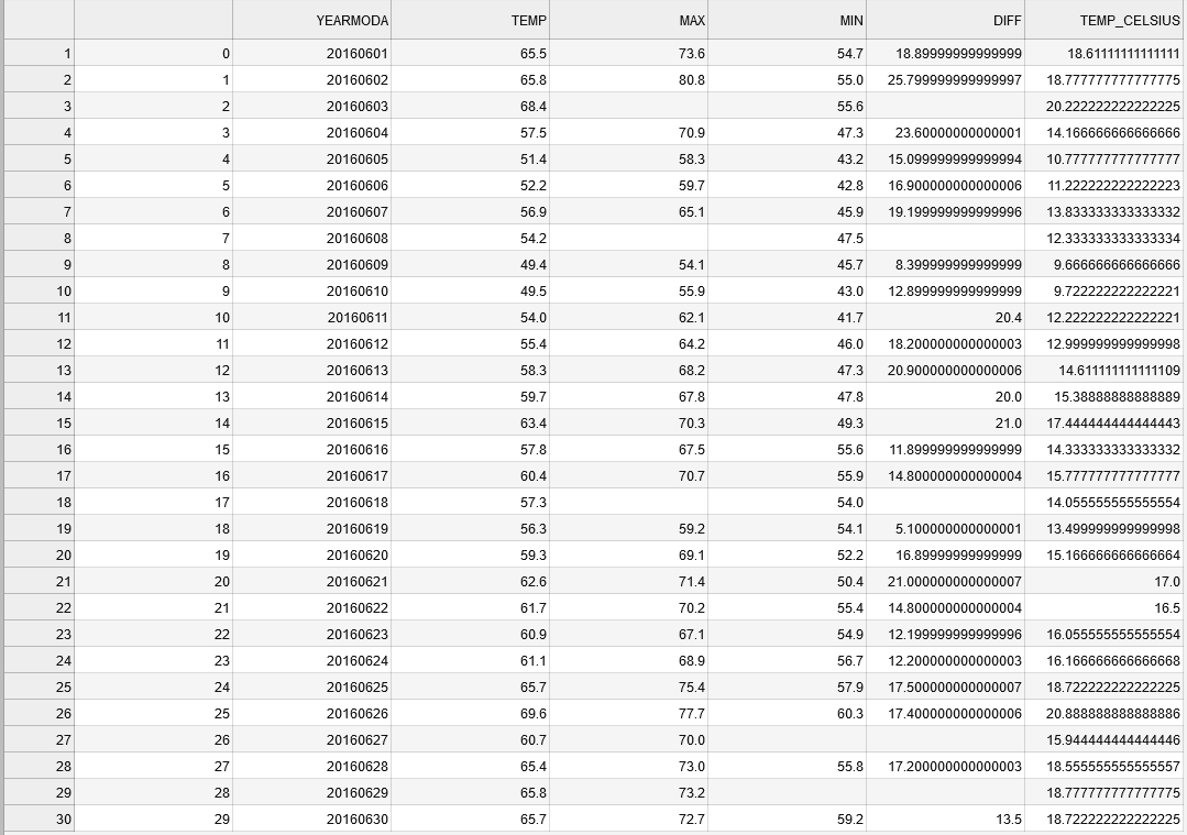
Let's update the column DIFF by calculating the difference between MAX and MIN columns to get an idea how much the temperatures have varied during the set of days:
# Calculate max min difference
data["DIFF"] = data["MAX"] - data["MIN"]

# Check the result
data.head()
The calculations were stored into the DIFF column as planned.
You can also create new columns on-the-fly at the same time when doing the calculation (the column does not have to exist before). Furthermore, it is possible to use any kind of math operation (e.g., subtraction, addition, multiplication, division, exponentiation, etc.) when creating new columns.
We can, for example, convert the Fahrenheit temperatures in the TEMP column to Celsius using the formula that we have already seen in this course many times. Let's do that and store it in a new column called TEMP_CELSIUS.
# Create a new column and convert temp fahrenheit to celsius:
data["TEMP_CELSIUS"] = (data["TEMP"] - 32) / (9 / 5)

# Check output
data.head()
# Solution
data["TEMP_KELVIN"] = data["TEMP_CELSIUS"] + 273.15
data.head()
Selecting rows and columns
We often want to select only specific rows from a DataFrame for further analysis. There are multiple ways of selecting subsets of a pandas DataFrame. In this section we will go through the most useful approaches for selecting specific rows, columns and individual values.
Selecting several rows
One common way of selecting only specific rows from your DataFrame is done via index slicing to extract part of the DataFrame. Slicing in pandas can be done in a similar manner as with normal Python lists (i.e., you specify the index range you want to select inside the square brackets): dataframe[start_index:stop_index].
Let's select the first five rows and assign them to a variable called selection:
# Select first five rows of dataframe using row index values
selection = data[0:5]
selection
{note}
Here we have selected the first five rows (index 0-4) using the integer index.
Selecting several rows and columns
It is also possible to control which columns are chosen when selecting a subset of rows. In this case we will use pandas.DataFrame.loc which selects data based on axis labels (row labels and column labels).
Let's select temperature values (column TEMP) from rows 0-5:
# Select temp column values on rows 0-5
selection = data.loc[0:5, "TEMP"]
selection
{note}
In this case, we get six rows of data (index 0-5)! We are now doing the selection based on axis labels instead of the integer index.
It is also possible to select multiple columns when using loc. Here, we select the TEMP and TEMP_CELSIUS columns from a set of rows by passing them inside a list (.loc[start_index:stop_index, list_of_columns]):
# Select columns temp and temp_celsius on rows 0-5
selection = data.loc[0:5, ["TEMP", "TEMP_CELSIUS"]]
selection
Check your understanding
Find the mean temperatures (in Celsius) for the last seven days of June. Do the selection using the row index values.
# Here is the solution
data.loc[23:29, "TEMP_CELSIUS"].mean()
Selecting a single row
You can also select an individual row from a specific position using the .loc[] indexing. Here we select all the data values using index 4 (the 5th row):
# Select one row using index
row = data.loc[4]
row
.loc[] indexing returns the values from that position as a pd.Series where the indices are actually the column names of those variables. Hence, you can access the value of an individual column by referring to its index using the following format (both should work):
# Print one attribute from the selected row
row["TEMP"]
Selecting a single value based on row and column
Sometimes it is enough to access a single value in a DataFrame. In this case, we can use DataFrame.at instead of Data.Frame.loc.
Let's select the temperature (column TEMP) on the first row (index 0) of our DataFrame.
data.at[0, "TEMP"]
Selections by integer position (optional)
{admonition}
`.loc` and `.at` are based on the *axis labels*, the names of columns and rows. Axis labels can also be something other than the "traditional" index values (e.g., `0`, `1`, ...). For example, datetime is commonly used as the row index for rows listed according to the date and time of the data.

`.iloc` is another indexing operator which is based on *integer value* indices. Using `.iloc`, it is possible to refer also to the columns based on their index value. For example,  `data.iloc[0,0]` would return `20160601` in our example DataFrame.

See the pandas documentation for more information about [indexing and selecting data](https://pandas.pydata.org/pandas-docs/stable/user_guide/indexing.html#indexing-and-selecting-data).
For example, we could select TEMP and the TEMP_CELSIUS columns from a set of rows based on their index.
data.iloc[0:5:, 0:2]
To access the value on the first row and second column (TEMP), the syntax for iloc would be:
data.iloc[0, 1]
We can also access individual rows using iloc. Let's check out the last row of data:
data.iloc[-1]
Filtering and updating data
One really useful feature in pandas is the ability to easily filter and select rows based on a conditional statement.
The following example shows how to select rows when the Celsius temperature has been higher than 15 degrees and store them in the variable warm_temps (warm temperatures). pandas checks if the condition is True or False for each row, and returns those rows where the condition is True:
# Check the condition
data["TEMP_CELSIUS"] > 15
# Select rows with temp celsius higher than 15 degrees
warm_temps = data.loc[data["TEMP_CELSIUS"] > 15]
warm_temps
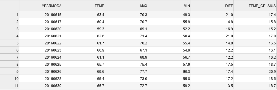
It is also possible to combine multiple criteria at the same time. Here, we select temperatures above 15 degrees that were recorded on the second half of June in 2016 (i.e. YEARMODA >= 20160615).
Combining multiple criteria can be done with the & operator (AND) or the | operator (OR). Notice, that it is often useful to separate the different clauses using parentheses ().
# Select rows with temp celsius higher than 15 degrees from late June 2016
warm_temps = data.loc[(data["TEMP_CELSIUS"] > 15) & (data["YEARMODA"] >= 20160615)]
warm_temps
Now we have a subset of our DataFrame with only rows where the TEMP_CELSIUS is above 15 and the dates in YEARMODA column start from the 15th of June.
Notice, that the index values (numbers on the left) are still showing the positions from the original DataFrame. It is possible to reset the index using the reset_index() function, which might be useful in some cases to be able to slice the data in a manner similar to that above. By default reset_index() would create a new column called index to keep track of the previous index, which might be useful in some cases. That is not hte case here, so we can omit that behavior by passing the parameter drop=True.
# Reset index
warm_temps = warm_temps.reset_index(drop=True)
warm_temps
As you can see, now the index values go from 0 to 12 now.
Check your understanding
Find the mean temperatures (in Celsius) for the last seven days of June again. This time you should select the rows based on a condition for the YEARMODA column!
# Here's the solution
data["TEMP_CELSIUS"].loc[data["YEARMODA"] >= 20160624].mean()
{admonition}
In this lesson, we have stored subsets of a DataFrame as a new variable. In some cases, we are still referring to the original data and any modifications made to the new variable might affect the original DataFrame.

If you want to be extra careful to not modify the original DataFrame, then you should take a *deep copy* of the data before proceeding using the `.copy()` method. You can read more about indexing, selecting data and deep and shallow copies in the [pandas documentation](https://pandas.pydata.org/pandas-docs/stable/user_guide/indexing.html) and in [this excellent blog post](https://medium.com/dunder-data/selecting-subsets-of-data-in-pandas-part-4-c4216f84d388).
Dealing with missing data
As you may have noticed by now, we have several missing values in the temperature minimum, maximum, and difference columns (MIN, MAX, and DIFF). These missing values are indicated as NaN (not a number). Having missing data in your datafile is a common situation and typically you want to deal with it somehow. Common procedures to deal with NaN values are to either remove them from the DataFrame or fill them with some other value. In pandas both of these options are easy to do.
Let's first see how we can remove the NoData values (i.e., clean the data) using the .dropna() function. Inside the function you can pass a list of column(s) from which the NaN values should found using the subset parameter. The output will drop any row containing NaN values from the set of columns provided to the subset parameter.
# Drop NaN values based on the MIN column
warm_temps_clean = warm_temps.dropna(subset=["MIN"])
warm_temps_clean
As you can see by looking at the table above (and the change in index values), we now have a DataFrame without the NoData values.
{note}
Note that we replaced the original `warm_temps` variable with version where no data are removed. The `.dropna()` function, among other pandas functions can also be applied "inplace" which means that the function updates the DataFrame object and returns `None`:

```python
warm_temps.dropna(subset=['MIN'], inplace=True)
```
Another option is to fill the NoData with some value using the fillna() function. Here we can fill the missing values in the with value -9999. Note that we are not giving the subset parameter this time.
# Fill NaN values
warm_temps.fillna(-9999)
As a result we now have a DataFrame where NoData values are filled with the value -9999.
{warning}
In many cases filling the data with a specific value is dangerous because you end up modifying the actual data, which might affect the results of your analysis. For example, in the case above we would have dramatically changed the temperature difference columns because the -9999 values not an actual temperature difference! Hence, use caution when filling missing values.

You might have to fill in no data values for the purposes of saving the data to file in a specific format. For example, some GIS software does not accept missing values. Always pay attention to potential no data values when reading in data files and doing further analysis!
Data type conversions
There are occasions where you'll need to convert data stored within a Series to another data type, for example, from floating point to integer.
Remember, that we already did data type conversions using the built-in Python functions such as int() or str().
For values in pandas DataFrames and Series, we can use the astype() method.
{admonition}
**Be careful with type conversions from floating point values to integers.** The conversion simply drops the stuff to the right of the decimal point, so all values are rounded down to the nearest whole number. For example, 99.99 will be truncated to 99 as an integer, when it should be rounded up to 100.

Chaining the round and type conversion functions solves this issue as the `.round(0).astype(int)` command first rounds the values with zero decimals and then converts those values into integers.
print("Original values:")
data["TEMP"].head()
print("Truncated integer values:")
data["TEMP"].astype(int).head()
print("Rounded integer values:")
data["TEMP"].round(0).astype(int).head()
Looks correct now.
Unique values
Sometimes it is useful to extract the unique values that you have in your column.
We can do that by using the unique() method:
# Get unique celsius values
unique = data["TEMP"].unique()
unique
As a result we get an array of unique values in that column.
{note}
Sometimes if you have a long list of unique values, you don't necessarily see all the unique values directly as IPython/Jupyter may hide them with an ellipsis `...`. It is, however, possible to see all those values by printing them as a list.
# unique values as list
list(unique)
How many days with unique mean temperature did we have in June 2016? We can check that!
# Number of unique values
unique_temps = len(unique)
print(f"There were {unique_temps} days with unique mean temperatures in June 2016.")
Sorting data
Quite often it is useful to be able to sort your data (descending/ascending) based on values in some column
This can be easily done with pandas using the sort_values(by='YourColumnName') function.
Let's first sort the values on ascending order based on the TEMP column:
# Sort DataFrame by temperature, ascending
data.sort_values(by="TEMP")
Of course, it is also possible to sort them in descending order with ascending=False parameter:
# Sort DataFrame by temperature, descending
data.sort_values(by="TEMP", ascending=False)
Writing data to a file
Lastly, it is important to be able to write the data that you have analyzed to a file on your computer. This is really handy in pandas as it supports many different data formats by default.
The most typical output format by far is a CSV file. The function to_csv() can be used to easily save your data in the CSV format. Let's first save the data from our data DataFrame into a file called Kumpula_temp_results_June_2016.csv.
# define output filename
output_fp = "Kumpula_temps_June_2016.csv"

# Save dataframe to csv
data.to_csv(output_fp, sep=",")
Now we have the data from our DataFrame saved to a file:
As you can see, the first value in the data file now contains the index value of the rows. There are also quite a lot of decimals present in the new columns
that we created. Let's deal with these and save the temperature values from the warm_temps DataFrame without the index and with only 1 decimal for the floating point numbers.
# define output filename
output_fp2 = "Kumpula_temps_above15_June_2016.csv"

# Save dataframe to csv
warm_temps.to_csv(output_fp2, sep=",", index=False, float_format="%.1f")
Omitting the index can be done with the index=False parameter. Specifying how many decimals should be written can be done with the float_format parameter where the text %.1f instructs pandas to use 1 decimal in all columns when writing the data to a file (changing the value 1 to 2 would write 2 decimals, etc.)
As a result you have a "cleaner" output file without the index column, and with only 1 decimal for floating point numbers.
That's it for this week. We will dive deeper into data analysis with pandas in the Lesson 6.