In [1]:
%matplotlib inline
import pandas as pd
import numpy as np
import matplotlib.pyplot as plt
pd.set_option('max_columns', 50)
Reading data
CSV
In [2]:
# this would be a huge pain to load into a database
mo = pd.read_csv('data/mariano-rivera.csv')
mo.tail()
Out[2]:
| Year | Age | Tm | Lg | W | L | W-L% | ERA | G | GS | GF | CG | SHO | SV | IP | H | R | ER | HR | BB | IBB | SO | HBP | BK | WP | BF | ERA+ | WHIP | H/9 | HR/9 | BB/9 | SO/9 | SO/BB | Awards | |
|---|---|---|---|---|---|---|---|---|---|---|---|---|---|---|---|---|---|---|---|---|---|---|---|---|---|---|---|---|---|---|---|---|---|---|
| 14 | 2009 | 39 | NYY | AL | 3 | 3 | 0.500 | 1.76 | 66 | 0 | 55 | 0 | 0 | 44 | 66.1 | 48 | 14 | 13 | 7 | 12 | 1 | 72 | 1 | 0 | 1 | 257 | 262 | 0.905 | 6.5 | 0.9 | 1.6 | 9.8 | 6.00 | ASMVP-14 |
| 15 | 2010 | 40 | NYY | AL | 3 | 3 | 0.500 | 1.80 | 61 | 0 | 55 | 0 | 0 | 33 | 60.0 | 39 | 14 | 12 | 2 | 11 | 3 | 45 | 5 | 0 | 0 | 230 | 241 | 0.833 | 5.9 | 0.3 | 1.7 | 6.8 | 4.09 | AS |
| 16 | 2011 | 41 | NYY | AL | 1 | 2 | 0.333 | 1.91 | 64 | 0 | 54 | 0 | 0 | 44 | 61.1 | 47 | 13 | 13 | 3 | 8 | 2 | 60 | 2 | 0 | 1 | 233 | 226 | 0.897 | 6.9 | 0.4 | 1.2 | 8.8 | 7.50 | ASCYA-8 |
| 17 | 2012 | 42 | NYY | AL | 1 | 1 | 0.500 | 2.16 | 9 | 0 | 9 | 0 | 0 | 5 | 8.1 | 6 | 2 | 2 | 0 | 2 | 2 | 8 | 0 | 0 | 0 | 32 | 203 | 0.960 | 6.5 | 0.0 | 2.2 | 8.6 | 4.00 | NaN |
| 18 | 2013 | 43 | NYY | AL | 6 | 2 | 0.750 | 2.11 | 64 | 0 | 60 | 0 | 0 | 44 | 64.0 | 58 | 16 | 15 | 6 | 9 | 3 | 54 | 1 | 0 | 0 | 256 | 192 | 1.047 | 8.2 | 0.8 | 1.3 | 7.6 | 6.00 | AS |
URL
pandas can fetch data from a URL ...
In [3]:
clean = lambda s: s.replace('$', '')[:-1] if '.' in s else s.replace('$', '') # a lot going on here
url = 'https://raw.github.com/gjreda/best-sandwiches/master/data/best-sandwiches-geocode.tsv'
sandwiches = pd.read_table(url, sep='\t', converters={'price': lambda s: float(clean(s))})
sandwiches.head(3)
Out[3]:
| rank | sandwich | restaurant | description | price | address | city | phone | website | full_address | formatted_address | lat | lng | |
|---|---|---|---|---|---|---|---|---|---|---|---|---|---|
| 0 | 1 | BLT | Old Oak Tap | The B is applewood smoked—nice and snapp... | 10.0 | 2109 W. Chicago Ave. | Chicago | 773-772-0406 | theoldoaktap.com | 2109 W. Chicago Ave., Chicago | 2109 West Chicago Avenue, Chicago, IL 60622, USA | 41.895734 | -87.679960 |
| 1 | 2 | Fried Bologna | Au Cheval | Thought your bologna-eating days had retired w... | 9.0 | 800 W. Randolph St. | Chicago | 312-929-4580 | aucheval.tumblr.com | 800 W. Randolph St., Chicago | 800 West Randolph Street, Chicago, IL 60607, USA | 41.884672 | -87.647754 |
| 2 | 3 | Woodland Mushroom | Xoco | Leave it to Rick Bayless and crew to come up w... | 9.5 | 445 N. Clark St. | Chicago | 312-334-3688 | rickbayless.com | 445 N. Clark St., Chicago | 445 North Clark Street, Chicago, IL 60654, USA | 41.890602 | -87.630925 |
JSON
In [4]:
gh = pd.read_json('https://api.github.com/repos/pydata/pandas/issues?per_page=3')
gh[['body', 'created_at', 'title', 'url']].head(3)
Out[4]:
| body | created_at | title | url | |
|---|---|---|---|---|
| 0 | 2014-11-22 02:54:48 | DOC: Add where and mask to API doc | https://api.github.com/repos/pydata/pandas/iss... | |
| 1 | Related to #7979\r\n\r\nBecause `Index` is no ... | 2014-11-22 02:16:30 | API: Index.duplicated() should return `np.arra... | https://api.github.com/repos/pydata/pandas/iss... |
| 2 | I'm not sure if this is supported or not -- it... | 2014-11-21 19:49:36 | HDF corrupts data when using complib='blosc:zlib' | https://api.github.com/repos/pydata/pandas/iss... |
You'll likely need to do some parsing though - pandas read_json doesn't do well with nested JSON yet
Clipboard
Possibly my favorite way to read data into pandas ...
In [5]:
clip = pd.read_clipboard()
clip.head()
Out[5]:
| figsize=(16,8) |
|---|
SQL Database
In [6]:
# All of this is basically the same as it would be with Postgres, MySQL, or any other database
# Just pass pandas a connection object and it'll take care of the rest.
from pandas.io import sql
import sqlite3
conn = sqlite3.connect('data/towed.db')
query = "SELECT * FROM towed"
towed = sql.read_sql(query, con=conn, parse_dates={'date':'%m/%d/%Y'})
towed.head()
Out[6]:
| date | make | style | model | color | plate | state | towed_to | facility_phone | inventory_num | |
|---|---|---|---|---|---|---|---|---|---|---|
| 0 | 2014-11-18 | FORD | LL | BLK | S105053 | IL | 10300 S. Doty | (773) 568-8495 | 2750424 | |
| 1 | 2014-11-18 | HOND | 4D | ACC | BLK | S415270 | IL | 400 E. Lower Wacker | (312) 744-7550 | 917129 |
| 2 | 2014-11-18 | CHRY | VN | SIL | V847641 | IL | 701 N. Sacramento | (773) 265-7605 | 6798366 | |
| 3 | 2014-11-18 | HYUN | 4D | SIL | N756530 | IL | 400 E. Lower Wacker | (312) 744-7550 | 917127 | |
| 4 | 2014-11-18 | TOYT | 4D | WHI | K702211 | IL | 400 E. Lower Wacker | (312) 744-7550 | 917128 |
We're going to work with the towed dataset for a bit.
Inspecting
We've already been using .head(), but there's also .tail(). You can also use standard Python slicing.
In [7]:
towed[100:105]
Out[7]:
| date | make | style | model | color | plate | state | towed_to | facility_phone | inventory_num | |
|---|---|---|---|---|---|---|---|---|---|---|
| 100 | 2014-11-18 | FORD | 4D | SIL | B9455 | NB | 10300 S. Doty | (773) 568-8495 | 2750400 | |
| 101 | 2014-11-18 | BMW | 4D | WHI | V960806 | IL | 400 E. Lower Wacker | (312) 744-7550 | 917087 | |
| 102 | 2014-11-18 | DODG | PK | TK | RED | 1382871B | IL | 10300 S. Doty | (773) 568-8495 | 2750398 |
| 103 | 2014-11-18 | CHEV | 4D | TAN | V356714 | IL | 10300 S. Doty | (773) 568-8495 | 2750397 | |
| 104 | 2014-11-18 | BUIC | 4D | WHI | S941660 | IL | 10300 S. Doty | (773) 568-8495 | 2750396 |
In [8]:
towed.info() # empty string showing up as non-null value
<class 'pandas.core.frame.DataFrame'>
Int64Index: 5065 entries, 0 to 5064
Data columns (total 10 columns):
date              5065 non-null datetime64[ns]
make              5065 non-null object
style             5065 non-null object
model             5065 non-null object
color             5065 non-null object
plate             5065 non-null object
state             5065 non-null object
towed_to          5065 non-null object
facility_phone    5065 non-null object
inventory_num     5065 non-null int64
dtypes: datetime64[ns](1), int64(1), object(8)
memory usage: 435.3+ KB
In [9]:
mo.info() # note the nulls in the Awards column
<class 'pandas.core.frame.DataFrame'>
Int64Index: 19 entries, 0 to 18
Data columns (total 34 columns):
Year      19 non-null int64
Age       19 non-null int64
Tm        19 non-null object
Lg        19 non-null object
W         19 non-null int64
L         19 non-null int64
W-L%      19 non-null float64
ERA       19 non-null float64
G         19 non-null int64
GS        19 non-null int64
GF        19 non-null int64
CG        19 non-null int64
SHO       19 non-null int64
SV        19 non-null int64
IP        19 non-null float64
H         19 non-null int64
R         19 non-null int64
ER        19 non-null int64
HR        19 non-null int64
BB        19 non-null int64
IBB       19 non-null int64
SO        19 non-null int64
HBP       19 non-null int64
BK        19 non-null int64
WP        19 non-null int64
BF        19 non-null int64
ERA+      19 non-null int64
WHIP      19 non-null float64
H/9       19 non-null float64
HR/9      19 non-null float64
BB/9      19 non-null float64
SO/9      19 non-null float64
SO/BB     19 non-null float64
Awards    15 non-null object
dtypes: float64(9), int64(22), object(3)
memory usage: 5.2+ KB
In [10]:
mo.describe() # basic stats for any numeric column
Out[10]:
| Year | Age | W | L | W-L% | ERA | G | GS | GF | CG | SHO | SV | IP | H | R | ER | HR | BB | IBB | SO | HBP | BK | WP | BF | ERA+ | WHIP | H/9 | HR/9 | BB/9 | SO/9 | SO/BB | |
|---|---|---|---|---|---|---|---|---|---|---|---|---|---|---|---|---|---|---|---|---|---|---|---|---|---|---|---|---|---|---|---|
| count | 19.000000 | 19.000000 | 19.000000 | 19.000000 | 19.000000 | 19.000000 | 19.000000 | 19.000000 | 19.000000 | 19 | 19 | 19.000000 | 19.000000 | 19.000000 | 19.000000 | 19.000000 | 19.000000 | 19.000000 | 19.000000 | 19.000000 | 19.000000 | 19.000000 | 19.000000 | 19.000000 | 19.000000 | 19.000000 | 19.000000 | 19.000000 | 19.000000 | 19.000000 | 19.000000 |
| mean | 2004.000000 | 34.000000 | 4.315789 | 3.157895 | 0.570158 | 2.222105 | 58.684211 | 0.526316 | 50.105263 | 0 | 0 | 34.315789 | 67.315789 | 52.526316 | 17.894737 | 16.578947 | 3.736842 | 15.052632 | 2.157895 | 61.736842 | 2.421053 | 0.157895 | 0.684211 | 268.578947 | 222.157895 | 0.998684 | 6.994737 | 0.489474 | 1.994737 | 8.142105 | 4.870000 |
| std | 5.627314 | 5.627314 | 2.083070 | 1.462994 | 0.174293 | 0.918861 | 17.023032 | 2.294157 | 19.944074 | 0 | 0 | 15.198877 | 18.657506 | 15.886292 | 8.305920 | 8.064434 | 2.423086 | 8.140937 | 1.500487 | 24.250641 | 1.894899 | 0.374634 | 0.749269 | 75.045405 | 56.108291 | 0.171747 | 1.107787 | 0.328117 | 0.779939 | 1.403296 | 2.553853 |
| min | 1995.000000 | 25.000000 | 1.000000 | 0.000000 | 0.200000 | 1.380000 | 9.000000 | 0.000000 | 2.000000 | 0 | 0 | 0.000000 | 8.100000 | 6.000000 | 2.000000 | 2.000000 | 0.000000 | 2.000000 | 0.000000 | 8.000000 | 0.000000 | 0.000000 | 0.000000 | 32.000000 | 84.000000 | 0.665000 | 5.200000 | 0.000000 | 0.800000 | 5.300000 | 1.700000 |
| 25% | 1999.500000 | 29.500000 | 3.000000 | 2.000000 | 0.500000 | 1.800000 | 61.000000 | 0.000000 | 51.500000 | 0 | 0 | 31.500000 | 62.550000 | 45.000000 | 14.000000 | 13.000000 | 2.500000 | 10.500000 | 1.000000 | 51.500000 | 1.000000 | 0.000000 | 0.000000 | 251.000000 | 192.000000 | 0.901000 | 6.300000 | 0.300000 | 1.300000 | 6.900000 | 3.350000 |
| 50% | 2004.000000 | 34.000000 | 4.000000 | 3.000000 | 0.571000 | 1.910000 | 64.000000 | 0.000000 | 57.000000 | 0 | 0 | 39.000000 | 70.200000 | 58.000000 | 16.000000 | 14.000000 | 3.000000 | 12.000000 | 2.000000 | 60.000000 | 2.000000 | 0.000000 | 1.000000 | 277.000000 | 233.000000 | 0.994000 | 6.900000 | 0.400000 | 2.100000 | 8.000000 | 4.090000 |
| 75% | 2008.500000 | 38.500000 | 6.000000 | 4.000000 | 0.651500 | 2.250000 | 66.000000 | 0.000000 | 60.500000 | 0 | 0 | 44.000000 | 75.100000 | 63.000000 | 21.000000 | 19.000000 | 4.500000 | 19.000000 | 3.000000 | 73.000000 | 4.000000 | 0.000000 | 1.000000 | 303.500000 | 254.500000 | 1.070500 | 7.600000 | 0.600000 | 2.400000 | 9.250000 | 6.085000 |
| max | 2013.000000 | 43.000000 | 8.000000 | 6.000000 | 1.000000 | 5.510000 | 74.000000 | 10.000000 | 69.000000 | 0 | 0 | 53.000000 | 107.200000 | 73.000000 | 43.000000 | 41.000000 | 11.000000 | 34.000000 | 6.000000 | 130.000000 | 6.000000 | 1.000000 | 2.000000 | 425.000000 | 316.000000 | 1.507000 | 9.500000 | 1.500000 | 4.000000 | 10.900000 | 12.830000 |
Indexes
In [11]:
towed.set_index('date', inplace=True)
In [12]:
# SELECT *
# FROM towed
# WHERE date = '2014-11-04'
# LIMIT 5;
towed.ix['2014-11-04']
Out[12]:
| make | style | model | color | plate | state | towed_to | facility_phone | inventory_num | |
|---|---|---|---|---|---|---|---|---|---|
| date | |||||||||
| 2014-11-04 | LINC | LL | GRN | V322831 | IL | 10300 S. Doty | (773) 568-8495 | 2749375 | |
| 2014-11-04 | CHRY | VN | BLU | 7101535 | IL | 701 N. Sacramento | (773) 265-7605 | 6797250 | |
| 2014-11-04 | PLYM | VN | TK | GRN | V144454 | IL | 701 N. Sacramento | (773) 265-7605 | 6797248 |
| 2014-11-04 | CHEV | VN | TK | BLK | K719308 | IL | 701 N. Sacramento | (773) 265-7605 | 6797246 |
| 2014-11-04 | CHEV | 4D | IMP | SIL | UG5J2P | MO | 701 N. Sacramento | (773) 265-7605 | 6797244 |
| 2014-11-04 | FORD | SW | SIL | S860992 | IL | 10300 S. Doty | (773) 568-8495 | 2749362 | |
| 2014-11-04 | DODG | VN | RED | 571R990 | IL | 701 N. Sacramento | (773) 265-7605 | 6797239 | |
| 2014-11-04 | DODG | PK | TK | BRO | 1381812 | IL | 10300 S. Doty | (773) 568-8495 | 2749364 |
| 2014-11-04 | ZCZY | 2D | BRO | IL | 10300 S. Doty | (773) 785-9752 | 1714849 | ||
| 2014-11-04 | CHEV | 4D | SIL | 10300 S. Doty | (773) 568-8495 | 2749363 | |||
| 2014-11-04 | CHEV | 4D | BLK | K527576 | IL | 10300 S. Doty | (773) 568-8495 | 2749365 | |
| 2014-11-04 | OLDS | VN | TK | MAR | 695R324 | IL | 701 N. Sacramento | (773) 265-7605 | 6797237 |
| 2014-11-04 | OLDS | 4D | TAN | N646613 | IL | 10300 S. Doty | (773) 568-8495 | 2749359 | |
| 2014-11-04 | LINC | 4D | SIL | 10300 S. Doty | (773) 568-8495 | 2749358 | |||
| 2014-11-04 | LINC | 4D | BLK | E144539 | IN | 10300 S. Doty | (773) 785-9752 | 1714848 | |
| 2014-11-04 | ISU | LL | TK | WHI | AY82383 | AL | 701 N. Sacramento | (773) 265-7605 | 6797232 |
| 2014-11-04 | HYUN | 2T | GRN | S991561 | IL | 701 N. Sacramento | (773) 265-7605 | 6797224 | |
| 2014-11-04 | TOYT | VN | GRN | R620262 | IL | 701 N. Sacramento | (773) 265-7605 | 6797225 | |
| 2014-11-04 | CHEV | LL | GRY | IT9801M | IL | 10300 S. Doty | (773) 568-8495 | 2749335 | |
| 2014-11-04 | CHEV | 4D | BLK | R689805 | IL | 10300 S. Doty | (773) 568-8495 | 6797229 | |
| 2014-11-04 | SAA | 4D | BLK | V901738 | IL | 10300 S. Doty | (773) 785-9752 | 1714847 | |
| 2014-11-04 | PONT | 4D | MAR | X149084 | IL | 10300 S. Doty | (773) 785-9752 | 1714846 | |
| 2014-11-04 | DODG | 4D | GRY | IL | 10300 S. Doty | (773) 568-8495 | 2749357 | ||
| 2014-11-04 | NISS | 4D | BLK | S806552 | IL | 10300 S. Doty | (773) 568-8495 | 2749355 | |
| 2014-11-04 | DODG | 4D | GRY | P432676 | IL | 701 N. Sacramento | (773) 265-7605 | 6797220 | |
| 2014-11-04 | OLDS | 4D | BLK | IL | 701 N. Sacramento | (773) 265-7605 | 6797216 | ||
| 2014-11-04 | PONT | 4D | MAR | 837PDG | WI | 701 N. Sacramento | (773) 265-7605 | 6797217 | |
| 2014-11-04 | DODG | VN | RED | IL | 10300 S. Doty | (773) 568-8495 | 2749360 | ||
| 2014-11-04 | FORD | LL | BLK | V521737 | IL | 10300 S. Doty | (773) 568-8495 | 464577 | |
| 2014-11-04 | FORD | 4D | GRY | L702784 | IL | 10300 S. Doty | (773) 785-9752 | 1714845 | |
| ... | ... | ... | ... | ... | ... | ... | ... | ... | ... |
| 2014-11-04 | LINC | 4D | GRN | L901713 | IL | 10300 S. Doty | (773) 568-8495 | 2749370 | |
| 2014-11-04 | TOYT | 2D | SIL | 190R367 | IL | 10300 S. Doty | (773) 568-8495 | 2749345 | |
| 2014-11-04 | TOYT | 2D | GRN | V241962 | IL | 10300 S. Doty | (773) 568-8495 | 2749352 | |
| 2014-11-04 | MASE | 4D | GRY | B345780 | IL | 701 N. Sacramento | (773) 265-7605 | 6797207 | |
| 2014-11-04 | DODG | VN | WHI | L293657 | IL | 10300 S. Doty | (773) 568-8495 | 2749354 | |
| 2014-11-04 | NISS | LL | GRY | V583736 | IL | 701 N. Sacramento | (773) 265-7605 | 6797201 | |
| 2014-11-04 | FORD | LL | BLK | 796ERG | MN | 701 N. Sacramento | (773) 265-1846 | 1532877 | |
| 2014-11-04 | FORD | LL | BLK | S485239 | IL | 10300 S. Doty | (773) 568-8495 | 2749349 | |
| 2014-11-04 | DODG | 4D | BLK | E274365 | IL | 10300 S. Doty | (773) 568-8495 | 2749348 | |
| 2014-11-04 | PONT | 4D | MAR | S728401 | IL | 10300 S. Doty | (773) 568-8495 | 2749347 | |
| 2014-11-04 | JEEP | LL | RED | R491482 | IL | 701 N. Sacramento | (773) 265-7605 | 6797196 | |
| 2014-11-04 | LINC | 4D | BLK | R470097 | IL | 701 N. Sacramento | (773) 265-7605 | 6797194 | |
| 2014-11-04 | FORD | 2D | WHI | V145161 | IL | 701 N. Sacramento | (773) 265-7605 | 6797188 | |
| 2014-11-04 | FORD | VN | WHI | 00527142 | IL | 701 N. Sacramento | (773) 265-7605 | 6797186 | |
| 2014-11-04 | DODG | 4D | SIL | P579868 | IL | 10300 S. Doty | (773) 568-8495 | 2749332 | |
| 2014-11-04 | FORD | 4D | DBL | CAPITAL | WI | 701 N. Sacramento | (773) 265-7605 | 6797189 | |
| 2014-11-04 | SATR | 4D | GRN | V514780 | IL | 701 N. Sacramento | (773) 265-7605 | 6797190 | |
| 2014-11-04 | OLDS | 4D | GRY | N935508 | IL | 10300 S. Doty | (773) 568-8495 | 2749343 | |
| 2014-11-04 | NISS | 4D | SIL | R952618 | IL | 10300 S. Doty | (773) 568-8495 | 2749329 | |
| 2014-11-04 | FORD | 4D | MAR | V612513 | IL | 10300 S. Doty | (773) 568-8495 | 2749337 | |
| 2014-11-04 | DODG | VN | TK | BLU | 731R563 | IL | 10300 S. Doty | (773) 568-8495 | 2749386 |
| 2014-11-04 | AUDI | 4D | WHI | E150919 | IL | 10300 S. Doty | (773) 568-8495 | 2749334 | |
| 2014-11-04 | PLYM | LL | GRY | IL | 10300 S. Doty | (773) 568-8495 | 2749326 | ||
| 2014-11-04 | FORD | 4D | GRN | VUO601 | IN | 701 N. Sacramento | (773) 265-7605 | 6797183 | |
| 2014-11-04 | CHEV | 4D | SIL | A014416 | IL | 701 N. Sacramento | (773) 265-7605 | 6797182 | |
| 2014-11-04 | INFI | 4D | BLK | V682152 | IL | 701 N. Sacramento | (773) 265-7605 | 6797178 | |
| 2014-11-04 | SUZI | LL | TAN | E259378 | IL | 701 N. Sacramento | (773) 265-7605 | 6797177 | |
| 2014-11-04 | MASE | 4D | GRY | IL | 10300 S. Doty | (773) 568-8495 | 2749377 | ||
| 2014-11-04 | CHEV | 2D | BLU | V609354 | IL | 10300 S. Doty | (773) 568-8495 | 2749378 | |
| 2014-11-04 | CHEV | 2D | SIL | 552P849 | IL | 10300 S. Doty | (773) 568-8495 | 2749381 |
70 rows × 9 columns
In [13]:
towed.ix['2014-11-04', 'make'] # get a Series back (or individual values, if unique)
Out[13]:
date
2014-11-04    LINC
2014-11-04    CHRY
2014-11-04    PLYM
2014-11-04    CHEV
2014-11-04    CHEV
2014-11-04    FORD
2014-11-04    DODG
2014-11-04    DODG
2014-11-04    ZCZY
2014-11-04    CHEV
2014-11-04    CHEV
2014-11-04    OLDS
2014-11-04    OLDS
2014-11-04    LINC
2014-11-04    LINC
...
2014-11-04    FORD
2014-11-04    SATR
2014-11-04    OLDS
2014-11-04    NISS
2014-11-04    FORD
2014-11-04    DODG
2014-11-04    AUDI
2014-11-04    PLYM
2014-11-04    FORD
2014-11-04    CHEV
2014-11-04    INFI
2014-11-04    SUZI
2014-11-04    MASE
2014-11-04    CHEV
2014-11-04    CHEV
Name: make, Length: 70
In [14]:
# SELECT *
# FROM towed
# WHERE date = '2014-11-04';
towed.reset_index(inplace=True)
towed[towed['date'] == '2014-11-04']
Out[14]:
| date | make | style | model | color | plate | state | towed_to | facility_phone | inventory_num | |
|---|---|---|---|---|---|---|---|---|---|---|
| 1350 | 2014-11-04 | LINC | LL | GRN | V322831 | IL | 10300 S. Doty | (773) 568-8495 | 2749375 | |
| 1351 | 2014-11-04 | CHRY | VN | BLU | 7101535 | IL | 701 N. Sacramento | (773) 265-7605 | 6797250 | |
| 1352 | 2014-11-04 | PLYM | VN | TK | GRN | V144454 | IL | 701 N. Sacramento | (773) 265-7605 | 6797248 |
| 1353 | 2014-11-04 | CHEV | VN | TK | BLK | K719308 | IL | 701 N. Sacramento | (773) 265-7605 | 6797246 |
| 1354 | 2014-11-04 | CHEV | 4D | IMP | SIL | UG5J2P | MO | 701 N. Sacramento | (773) 265-7605 | 6797244 |
| 1355 | 2014-11-04 | FORD | SW | SIL | S860992 | IL | 10300 S. Doty | (773) 568-8495 | 2749362 | |
| 1356 | 2014-11-04 | DODG | VN | RED | 571R990 | IL | 701 N. Sacramento | (773) 265-7605 | 6797239 | |
| 1357 | 2014-11-04 | DODG | PK | TK | BRO | 1381812 | IL | 10300 S. Doty | (773) 568-8495 | 2749364 |
| 1358 | 2014-11-04 | ZCZY | 2D | BRO | IL | 10300 S. Doty | (773) 785-9752 | 1714849 | ||
| 1359 | 2014-11-04 | CHEV | 4D | SIL | 10300 S. Doty | (773) 568-8495 | 2749363 | |||
| 1360 | 2014-11-04 | CHEV | 4D | BLK | K527576 | IL | 10300 S. Doty | (773) 568-8495 | 2749365 | |
| 1361 | 2014-11-04 | OLDS | VN | TK | MAR | 695R324 | IL | 701 N. Sacramento | (773) 265-7605 | 6797237 |
| 1362 | 2014-11-04 | OLDS | 4D | TAN | N646613 | IL | 10300 S. Doty | (773) 568-8495 | 2749359 | |
| 1363 | 2014-11-04 | LINC | 4D | SIL | 10300 S. Doty | (773) 568-8495 | 2749358 | |||
| 1364 | 2014-11-04 | LINC | 4D | BLK | E144539 | IN | 10300 S. Doty | (773) 785-9752 | 1714848 | |
| 1365 | 2014-11-04 | ISU | LL | TK | WHI | AY82383 | AL | 701 N. Sacramento | (773) 265-7605 | 6797232 |
| 1366 | 2014-11-04 | HYUN | 2T | GRN | S991561 | IL | 701 N. Sacramento | (773) 265-7605 | 6797224 | |
| 1367 | 2014-11-04 | TOYT | VN | GRN | R620262 | IL | 701 N. Sacramento | (773) 265-7605 | 6797225 | |
| 1368 | 2014-11-04 | CHEV | LL | GRY | IT9801M | IL | 10300 S. Doty | (773) 568-8495 | 2749335 | |
| 1369 | 2014-11-04 | CHEV | 4D | BLK | R689805 | IL | 10300 S. Doty | (773) 568-8495 | 6797229 | |
| 1370 | 2014-11-04 | SAA | 4D | BLK | V901738 | IL | 10300 S. Doty | (773) 785-9752 | 1714847 | |
| 1371 | 2014-11-04 | PONT | 4D | MAR | X149084 | IL | 10300 S. Doty | (773) 785-9752 | 1714846 | |
| 1372 | 2014-11-04 | DODG | 4D | GRY | IL | 10300 S. Doty | (773) 568-8495 | 2749357 | ||
| 1373 | 2014-11-04 | NISS | 4D | BLK | S806552 | IL | 10300 S. Doty | (773) 568-8495 | 2749355 | |
| 1374 | 2014-11-04 | DODG | 4D | GRY | P432676 | IL | 701 N. Sacramento | (773) 265-7605 | 6797220 | |
| 1375 | 2014-11-04 | OLDS | 4D | BLK | IL | 701 N. Sacramento | (773) 265-7605 | 6797216 | ||
| 1376 | 2014-11-04 | PONT | 4D | MAR | 837PDG | WI | 701 N. Sacramento | (773) 265-7605 | 6797217 | |
| 1377 | 2014-11-04 | DODG | VN | RED | IL | 10300 S. Doty | (773) 568-8495 | 2749360 | ||
| 1378 | 2014-11-04 | FORD | LL | BLK | V521737 | IL | 10300 S. Doty | (773) 568-8495 | 464577 | |
| 1379 | 2014-11-04 | FORD | 4D | GRY | L702784 | IL | 10300 S. Doty | (773) 785-9752 | 1714845 | |
| ... | ... | ... | ... | ... | ... | ... | ... | ... | ... | ... |
| 1390 | 2014-11-04 | LINC | 4D | GRN | L901713 | IL | 10300 S. Doty | (773) 568-8495 | 2749370 | |
| 1391 | 2014-11-04 | TOYT | 2D | SIL | 190R367 | IL | 10300 S. Doty | (773) 568-8495 | 2749345 | |
| 1392 | 2014-11-04 | TOYT | 2D | GRN | V241962 | IL | 10300 S. Doty | (773) 568-8495 | 2749352 | |
| 1393 | 2014-11-04 | MASE | 4D | GRY | B345780 | IL | 701 N. Sacramento | (773) 265-7605 | 6797207 | |
| 1394 | 2014-11-04 | DODG | VN | WHI | L293657 | IL | 10300 S. Doty | (773) 568-8495 | 2749354 | |
| 1395 | 2014-11-04 | NISS | LL | GRY | V583736 | IL | 701 N. Sacramento | (773) 265-7605 | 6797201 | |
| 1396 | 2014-11-04 | FORD | LL | BLK | 796ERG | MN | 701 N. Sacramento | (773) 265-1846 | 1532877 | |
| 1397 | 2014-11-04 | FORD | LL | BLK | S485239 | IL | 10300 S. Doty | (773) 568-8495 | 2749349 | |
| 1398 | 2014-11-04 | DODG | 4D | BLK | E274365 | IL | 10300 S. Doty | (773) 568-8495 | 2749348 | |
| 1399 | 2014-11-04 | PONT | 4D | MAR | S728401 | IL | 10300 S. Doty | (773) 568-8495 | 2749347 | |
| 1400 | 2014-11-04 | JEEP | LL | RED | R491482 | IL | 701 N. Sacramento | (773) 265-7605 | 6797196 | |
| 1401 | 2014-11-04 | LINC | 4D | BLK | R470097 | IL | 701 N. Sacramento | (773) 265-7605 | 6797194 | |
| 1402 | 2014-11-04 | FORD | 2D | WHI | V145161 | IL | 701 N. Sacramento | (773) 265-7605 | 6797188 | |
| 1403 | 2014-11-04 | FORD | VN | WHI | 00527142 | IL | 701 N. Sacramento | (773) 265-7605 | 6797186 | |
| 1404 | 2014-11-04 | DODG | 4D | SIL | P579868 | IL | 10300 S. Doty | (773) 568-8495 | 2749332 | |
| 1405 | 2014-11-04 | FORD | 4D | DBL | CAPITAL | WI | 701 N. Sacramento | (773) 265-7605 | 6797189 | |
| 1406 | 2014-11-04 | SATR | 4D | GRN | V514780 | IL | 701 N. Sacramento | (773) 265-7605 | 6797190 | |
| 1407 | 2014-11-04 | OLDS | 4D | GRY | N935508 | IL | 10300 S. Doty | (773) 568-8495 | 2749343 | |
| 1408 | 2014-11-04 | NISS | 4D | SIL | R952618 | IL | 10300 S. Doty | (773) 568-8495 | 2749329 | |
| 1409 | 2014-11-04 | FORD | 4D | MAR | V612513 | IL | 10300 S. Doty | (773) 568-8495 | 2749337 | |
| 1410 | 2014-11-04 | DODG | VN | TK | BLU | 731R563 | IL | 10300 S. Doty | (773) 568-8495 | 2749386 |
| 1411 | 2014-11-04 | AUDI | 4D | WHI | E150919 | IL | 10300 S. Doty | (773) 568-8495 | 2749334 | |
| 1412 | 2014-11-04 | PLYM | LL | GRY | IL | 10300 S. Doty | (773) 568-8495 | 2749326 | ||
| 1413 | 2014-11-04 | FORD | 4D | GRN | VUO601 | IN | 701 N. Sacramento | (773) 265-7605 | 6797183 | |
| 1414 | 2014-11-04 | CHEV | 4D | SIL | A014416 | IL | 701 N. Sacramento | (773) 265-7605 | 6797182 | |
| 1415 | 2014-11-04 | INFI | 4D | BLK | V682152 | IL | 701 N. Sacramento | (773) 265-7605 | 6797178 | |
| 1416 | 2014-11-04 | SUZI | LL | TAN | E259378 | IL | 701 N. Sacramento | (773) 265-7605 | 6797177 | |
| 1417 | 2014-11-04 | MASE | 4D | GRY | IL | 10300 S. Doty | (773) 568-8495 | 2749377 | ||
| 1418 | 2014-11-04 | CHEV | 2D | BLU | V609354 | IL | 10300 S. Doty | (773) 568-8495 | 2749378 | |
| 1419 | 2014-11-04 | CHEV | 2D | SIL | 552P849 | IL | 10300 S. Doty | (773) 568-8495 | 2749381 |
70 rows × 10 columns
In [15]:
towed.set_index('date', inplace=True)
Selection
In [16]:
cols = ['make', 'color', 'state'] # just passing a list
towed[cols][:5]
Out[16]:
| make | color | state | |
|---|---|---|---|
| date | |||
| 2014-11-18 | FORD | BLK | IL |
| 2014-11-18 | HOND | BLK | IL |
| 2014-11-18 | CHRY | SIL | IL |
| 2014-11-18 | HYUN | SIL | IL |
| 2014-11-18 | TOYT | WHI | IL |
Filtering
In [17]:
# SELECT *
# FROM towed
# WHERE make = 'FORD'
# ORDER BY state DESC
# LIMIT 5;
towed[towed['make'] == 'FORD'].sort('state', ascending=False).head()
Out[17]:
| make | style | model | color | plate | state | towed_to | facility_phone | inventory_num | |
|---|---|---|---|---|---|---|---|---|---|
| date | |||||||||
| 2014-11-04 | FORD | 4D | DBL | CAPITAL | WI | 701 N. Sacramento | (773) 265-7605 | 6797189 | |
| 2014-10-22 | FORD | 4D | TAU | RED | 113WDP | WI | 701 N. Sacramento | (773) 265-7605 | 6796198 |
| 2014-11-08 | FORD | LL | BLK | 635FJE | WI | 10300 S. Doty | (773) 568-8495 | 2749537 | |
| 2014-10-06 | FORD | 2D | ONG | 198WJX | WI | 701 N. Sacramento | (773) 265-7605 | 6794908 | |
| 2014-11-10 | FORD | 4D | BLU | 250WLU | WI | 701 N. Sacramento | (773) 265-7605 | 6797787 |
In [18]:
# SELECT *
# FROM towed
# WHERE color = 'BLK'
#   AND state = 'MI';
towed[(towed.color == 'BLK') & (towed.state == 'MI')]
Out[18]:
| make | style | model | color | plate | state | towed_to | facility_phone | inventory_num | |
|---|---|---|---|---|---|---|---|---|---|
| date | |||||||||
| 2014-11-12 | DODG | LL | BLK | CLV6160 | MI | 701 N. Sacramento | (773) 265-7605 | 6797946 | |
| 2014-09-08 | CHEV | 2D | BLK | 3KMT29 | MI | 10300 S. Doty | (773) 568-8495 | 2745448 | |
| 2014-08-27 | KIA | 4D | BLK | DAN1057 | MI | 701 N. Sacramento | (773) 265-7605 | 6791554 |
In [19]:
# SELECT *
# FROM towed
# WHERE make = 'PORS'
#   OR state = 'NY'
# ORDER BY make, color DESC;
towed[(towed.make == 'PORS') | (towed.state == 'NY')].sort(['make', 'color'], ascending=[True, False]) # not red Porshe
Out[19]:
| make | style | model | color | plate | state | towed_to | facility_phone | inventory_num | |
|---|---|---|---|---|---|---|---|---|---|
| date | |||||||||
| 2014-09-27 | AUDI | 4D | SIL | EWA7707 | NY | 701 N. Sacramento | (773) 265-7605 | 6794421 | |
| 2014-09-27 | AUDI | 4D | SIL | EWA7707 | NY | 701 N. Sacramento | (773) 265-7605 | 6794421 | |
| 2014-11-11 | BUIC | LL | WHI | GNW2480 | NY | 10300 S. Doty | (773) 568-8495 | 2749681 | |
| 2014-10-08 | PORS | LL | RED | V515513 | IL | 701 N. Sacramento | (773) 265-7605 | 6795116 | |
| 2014-11-01 | PORS | LL | BLK | V671447 | IL | 10300 S. Doty | (773) 568-8495 | 2749122 | |
| 2014-09-25 | PORS | LL | BLK | IL | 701 N. Sacramento | (773) 265-7605 | 6794214 | ||
| 2014-09-19 | PORS | LL | BLK | V733398 | IL | 701 N. Sacramento | (773) 265-7605 | 6793740 | |
| 2014-09-01 | SUZI | 4D | GRY | EHL9836 | NY | 10300 S. Doty | (773) 568-8495 | 2744842 |
In [20]:
m = (towed.style == '4D') & (towed.state == 'IL') # create a filter mask
In [21]:
m.value_counts() # it's just a boolean series
Out[21]:
True     2570
False    2495
dtype: int64
In [22]:
# SELECT make, model, color
# FROM towed
# WHERE style = '4D' AND state = 'IL
# ORDER BY date
# LIMIT 5;
towed[m][['make', 'model', 'color']].sort().head()
Out[22]:
| make | model | color | |
|---|---|---|---|
| date | |||
| 2014-08-20 | BUIC | GRY | |
| 2014-08-20 | LEXS | BLK | |
| 2014-08-21 | NISS | GRY | |
| 2014-08-21 | HOND | GRY | |
| 2014-08-21 | PONT | BLK |
In [23]:
towed[towed.duplicated()] # this would suck in SQL ... but that's also what primary keys are for
Out[23]:
| make | style | model | color | plate | state | towed_to | facility_phone | inventory_num | |
|---|---|---|---|---|---|---|---|---|---|
| date | |||||||||
| 2014-11-18 | NISS | 4D | GRY | E203840 | IL | 400 E. Lower Wacker | (312) 744-7550 | 6798305 | |
| 2014-11-06 | BUIC | 4D | PLE | R4548 | IL | 701 N. Sacramento | (773) 265-7605 | 6797394 | |
| 2014-11-03 | FORD | 4D | BLK | S227831 | IL | 10300 S. Doty | (773) 568-8495 | 2749299 | |
| 2014-10-19 | MERZ | LL | TK | BLK | MINE-IP | IL | 701 N. Sacramento | (773) 265-7605 | 6795998 |
| 2014-10-11 | FORD | LL | RED | IL | 10300 S. Doty | (773) 568-8495 | 2747534 | ||
| 2014-09-27 | AUDI | 4D | SIL | EWA7707 | NY | 701 N. Sacramento | (773) 265-7605 | 6794421 | |
| 2014-09-04 | CHEV | 4D | LUM | WHI | S880655 | IL | 10300 S. Doty | (773) 568-8495 | 2745054 |
| 2014-09-03 | CHEV | LL | GRY | K585960 | IL | 10300 S. Doty | (773) 568-8495 | 2744980 |
In [24]:
# thousands comma in tripduration field ... that's be really annoying to load into a DB
! egrep \"[0-9],[0-9]+\" data/divvy/Divvy_Trips_2013.csv | head -n 5
In [25]:
! head -n 5 data/divvy/Divvy_Stations_2013.csv
In [26]:
! head -n 5 data/weather.csv
CDT,Max TemperatureF,Mean TemperatureF,Min TemperatureF,Max Dew PointF,MeanDew PointF,Min DewpointF,Max Humidity, Mean Humidity, Min Humidity, Max Sea Level PressureIn, Mean Sea Level PressureIn, Min Sea Level PressureIn, Max VisibilityMiles, Mean VisibilityMiles, Min VisibilityMiles, Max Wind SpeedMPH, Mean Wind SpeedMPH, Max Gust SpeedMPH,PrecipitationIn, CloudCover, Events, WindDirDegrees
2013-6-1,76,70,63,70,63,61,93,81,68,29.73,29.69,29.66,10,9,2,25,13,33,0.56,7,Rain-Thunderstorm,213
2013-6-2,63,53,43,59,50,42,97,84,71,30.04,29.92,29.71,10,9,3,16,6,23,0.01,6,Rain,63
2013-6-3,68,56,43,46,42,38,100,69,37,30.12,30.07,30.04,10,10,10,14,5,20,0.00,2,,142
2013-6-4,72,61,50,49,45,41,93,64,35,30.16,30.12,30.09,10,10,10,14,6,21,0.00,5,,73
In [27]:
from datetime import datetime
to_datetime = lambda d: datetime.strptime(d, '%m/%d/%Y %H:%M')
In [28]:
# if you know the datetime format, it's much, much faster to explicitly parse it
# see here: https://gist.github.com/gjreda/7433f5f70299610d9b6b
trips = pd.read_csv('data/divvy/Divvy_Trips_2013.csv',
                    converters={'starttime': to_datetime,'stoptime': to_datetime},
                    thousands=',')
stations = pd.read_csv('data/divvy/Divvy_Stations_2013.csv')
/Users/gjreda/.virtualenvs/pydata2014/lib/python2.7/site-packages/pandas/io/parsers.py:1154: DtypeWarning: Columns (10) have mixed types. Specify dtype option on import or set low_memory=False.
  data = self._reader.read(nrows)
In [29]:
trips.info()
<class 'pandas.core.frame.DataFrame'>
Int64Index: 759788 entries, 0 to 759787
Data columns (total 12 columns):
trip_id              759788 non-null int64
starttime            759788 non-null datetime64[ns]
stoptime             759788 non-null datetime64[ns]
bikeid               759788 non-null int64
tripduration         759788 non-null int64
from_station_id      758826 non-null float64
from_station_name    759788 non-null object
to_station_id        758829 non-null float64
to_station_name      759788 non-null object
usertype             759788 non-null object
gender               403046 non-null object
birthyear            402909 non-null float64
dtypes: datetime64[ns](2), float64(3), int64(3), object(4)
memory usage: 75.4+ MB
In [30]:
stations.info()
<class 'pandas.core.frame.DataFrame'>
Int64Index: 300 entries, 0 to 299
Data columns (total 4 columns):
name          300 non-null object
latitude      300 non-null float64
longitude     300 non-null float64
dpcapacity    300 non-null int64
dtypes: float64(2), int64(1), object(1)
memory usage: 11.7+ KB

LEFT JOIN
In [31]:
# CREATE TABLE divvy (
#   SELECT *
#   FROM trips
#   LEFT JOIN stations
#     ON trips.from_station_name = stations.name
# );
divvy = pd.merge(trips, stations, how='left', left_on='from_station_name', right_on='name')
divvy.info()
<class 'pandas.core.frame.DataFrame'>
Int64Index: 759788 entries, 0 to 759787
Data columns (total 16 columns):
trip_id              759788 non-null int64
starttime            759788 non-null datetime64[ns]
stoptime             759788 non-null datetime64[ns]
bikeid               759788 non-null int64
tripduration         759788 non-null int64
from_station_id      758826 non-null float64
from_station_name    759788 non-null object
to_station_id        758829 non-null float64
to_station_name      759788 non-null object
usertype             759788 non-null object
gender               403046 non-null object
birthyear            402909 non-null float64
name                 759788 non-null object
latitude             759788 non-null float64
longitude            759788 non-null float64
dpcapacity           759788 non-null int64
dtypes: datetime64[ns](2), float64(5), int64(4), object(5)
memory usage: 98.5+ MB
In [32]:
# SELECT trip_id, ... divvy.name AS name_origin ... stations.name AS name_dest
# FROM divvy
# INNER JOIN stations
#   ON divvy.to_station_name = stations.name
divvy = pd.merge(divvy, stations, how='inner', left_on='to_station_name', right_on='name', suffixes=['_origin', '_dest'])
divvy.info()
<class 'pandas.core.frame.DataFrame'>
Int64Index: 759788 entries, 0 to 759787
Data columns (total 20 columns):
trip_id              759788 non-null int64
starttime            759788 non-null datetime64[ns]
stoptime             759788 non-null datetime64[ns]
bikeid               759788 non-null int64
tripduration         759788 non-null int64
from_station_id      758826 non-null float64
from_station_name    759788 non-null object
to_station_id        758829 non-null float64
to_station_name      759788 non-null object
usertype             759788 non-null object
gender               403046 non-null object
birthyear            402909 non-null float64
name_origin          759788 non-null object
latitude_origin      759788 non-null float64
longitude_origin     759788 non-null float64
dpcapacity_origin    759788 non-null int64
name_dest            759788 non-null object
latitude_dest        759788 non-null float64
longitude_dest       759788 non-null float64
dpcapacity_dest      759788 non-null int64
dtypes: datetime64[ns](2), float64(7), int64(5), object(6)
memory usage: 121.7+ MB
UNION & UNION ALL (concatenation)
In [33]:
df1 = pd.DataFrame({'a': np.random.randn(3), 'b': np.square(range(100,103))})
df2 = pd.DataFrame({'a': [np.NaN, 11, 99], 'b': np.random.randn(3)})
In [34]:
# SELECT a, b
# FROM df1
# UNION
# SELECT a, b
# FROM df2;

# takes a list, so you can pass 2+ dataframes
# note that the indexes are the same
pd.concat([df1, df2])
Out[34]:
| a | b | |
|---|---|---|
| 0 | 0.200588 | 10000.000000 |
| 1 | 1.533702 | 10201.000000 |
| 2 | 0.977121 | 10404.000000 |
| 0 | NaN | -0.323561 |
| 1 | 11.000000 | -1.318334 |
| 2 | 99.000000 | -0.544382 |

In [35]:
# it's precise to the minute - want to see counts by nearest hour
divvy.starttime.value_counts().order()[:3]
Out[35]:
2013-11-21 19:05:00    1
2013-09-17 05:40:00    1
2013-12-21 20:17:00    1
dtype: int64
In [36]:
# I don't want to just extract the hour from the datetime ... NEAREST hour
from datetime import timedelta

def round_time(dt, mins=60):
    """
    Rounds a datetime object to its nearest hour (by default).
    (e.g. 2014-02-01 10:45:13 becomes 2014-02-01 11:00:00)
    """
    dt += timedelta(minutes=mins/2.)
    dt -= timedelta(minutes=dt.minute % mins, seconds=dt.second)
    return dt
In [37]:
divvy['starthour'] = divvy.starttime.apply(round_time)
divvy['stophour'] = divvy.stoptime.apply(round_time)
In [38]:
divvy[['starttime', 'starthour']].head(3)
Out[38]:
| starttime | starthour | |
|---|---|---|
| 0 | 2013-06-27 12:11:00 | 2013-06-27 12:00:00 |
| 1 | 2013-06-28 12:55:00 | 2013-06-28 13:00:00 |
| 2 | 2013-07-09 19:06:00 | 2013-07-09 19:00:00 |
Grouping
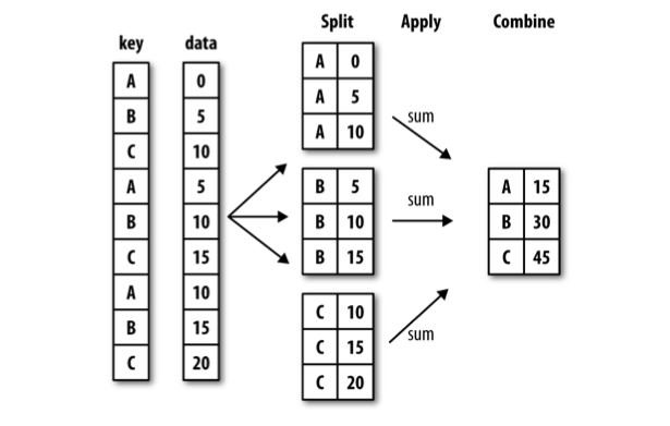
pandas groupby draws largely from Hadley Wickham's Split Apply Combine Methodology for Data Analysis (it's a good paper; you should read it).
Trips by starthour
Count vs Size
In [39]:
# SELECT starthour, count(1)
# FROM divvy
# GROUP BY starthour
divvy.groupby('starthour').size()
Out[39]:
starthour
2013-06-27 01:00:00     1
2013-06-27 11:00:00     3
2013-06-27 12:00:00     4
2013-06-27 13:00:00     2
2013-06-27 15:00:00    10
2013-06-27 16:00:00     2
2013-06-27 17:00:00     3
2013-06-27 18:00:00     1
2013-06-27 19:00:00    14
2013-06-27 20:00:00    21
2013-06-27 21:00:00     5
2013-06-27 22:00:00    17
2013-06-27 23:00:00     9
2013-06-28 00:00:00     8
2013-06-28 01:00:00     5
...
2013-12-31 10:00:00    20
2013-12-31 11:00:00    33
2013-12-31 12:00:00    47
2013-12-31 13:00:00    59
2013-12-31 14:00:00    52
2013-12-31 15:00:00    41
2013-12-31 16:00:00    43
2013-12-31 17:00:00    24
2013-12-31 18:00:00    12
2013-12-31 19:00:00     7
2013-12-31 20:00:00     7
2013-12-31 21:00:00     7
2013-12-31 22:00:00    12
2013-12-31 23:00:00     2
2014-01-01 00:00:00     2
Length: 4452
starthour with longest mean trip duration
In [40]:
# SELECT starthour, avg(tripduration)
# FROM divvy
# GROUP BY starthour
# ORDER BY avg(tripduration) DESC
# LIMIT 5
divvy.groupby('starthour')['tripduration'].mean().order(ascending=False)[:5]
Out[40]:
starthour
2013-06-27 01:00:00    31177.0
2013-06-28 02:00:00    28469.0
2013-07-24 03:00:00    24593.0
2013-12-18 02:00:00    22762.5
2013-07-22 04:00:00    21118.0
Name: tripduration, dtype: float64
Count of unique birthyears with mean and median tripduration by usertype
In [41]:
divvy.groupby('usertype').agg({'birthyear': pd.Series.nunique, 'tripduration': [np.mean, np.median]})
Out[41]:
| birthyear | tripduration | ||
|---|---|---|---|
| nunique | mean | median | |
| usertype | |||
| Customer | 4 | 1824.054727 | 1257 |
| Subscriber | 68 | 722.018892 | 566 |
Plotting
In [42]:
# number of trips started by starthour
divvy.groupby('starthour').size().plot(figsize=(16,8))
Out[42]:
<matplotlib.axes._subplots.AxesSubplot at 0x10bc9f4d0>

Distribution of trip duration
In [43]:
# distribution of tripduration
divvy.tripduration.hist(figsize=(16,8), bins=1000)
plt.xlim(0, 10000);

What percentage of Divvy rides are less than 10 minutes? 20 minutes?
Sounds like we need to plot the cumulative distribution of trip duration.
(If someone knows of a better way of doing this, I'd love to hear it).
In [44]:
duration_counts = divvy.tripduration.value_counts()
duration_counts.index.name = 'seconds'
duration_counts.name = 'trips'
duration_counts.head()
Out[44]:
seconds
408        712
399        711
346        706
379        701
415        700
Name: trips, dtype: int64
In [45]:
df = duration_counts.reset_index()
df['minutes'] = df.seconds/60.
df.set_index('minutes', inplace=True)
df.sort(inplace=True)
In [46]:
(df.trips.cumsum() / df.trips.sum()).plot(figsize=(16,8))
plt.xlim(0, 60)
plt.yticks(np.arange(0, 1.1, 0.1));

Number of trips per birth year
In [47]:
plt.figure(figsize=(9, 18))
divvy.groupby('birthyear').size().order().plot(kind='barh')
Out[47]:
<matplotlib.axes._subplots.AxesSubplot at 0x11072a5d0>

In [48]:
divvy.groupby(divvy['starttime'].apply(lambda d: d.dayofweek))['trip_id'].count().plot(kind='bar')
plt.title('Divvy trips by weekday') # 0 = Monday ...
plt.xlabel('Weekday')
plt.ylabel('# of trips started');

Men vs. Women
Plotting multiple lines and subplotting.
In [49]:
divvy['startdate'] = divvy.starthour.apply(lambda d: d.date())
by_gender = divvy.groupby(['startdate', 'gender']).size()
In [50]:
by_gender.head()
Out[50]:
startdate   gender
2013-06-27  Female     14
            Male       45
2013-06-28  Female     75
            Male      321
2013-06-29  Female     42
dtype: int64
In [51]:
by_gender.unstack(1).head()
Out[51]:
| gender | Female | Male |
|---|---|---|
| startdate | ||
| 2013-06-27 | 14 | 45 |
| 2013-06-28 | 75 | 321 |
| 2013-06-29 | 42 | 163 |
| 2013-06-30 | 47 | 180 |
| 2013-07-01 | 87 | 449 |
pandas wins here.
In [52]:
# SELECT startdate
#    , COUNT(IF(gender = 'Female', 1, NULL))
#    , COUNT(IF(gender = 'Male', 1, NULL))
# FROM divvy
# GROUP BY startdate
# LIMIT 5;
divvy.groupby(['startdate', 'gender']).size().unstack(1).head()
Out[52]:
| gender | Female | Male |
|---|---|---|
| startdate | ||
| 2013-06-27 | 14 | 45 |
| 2013-06-28 | 75 | 321 |
| 2013-06-29 | 42 | 163 |
| 2013-06-30 | 47 | 180 |
| 2013-07-01 | 87 | 449 |
In [53]:
by_gender.unstack(1).plot(figsize=(16,8))
Out[53]:
<matplotlib.axes._subplots.AxesSubplot at 0x1102ecf10>

Consumer vs Subscriber
In [54]:
divvy.groupby(['startdate', 'usertype']).size().unstack(1).plot(figsize=(16,8), subplots=True);

Trips by weekday hour
In [55]:
weekdays = divvy['starttime'].apply(lambda d: d.dayofweek)
hours = divvy['starttime'].apply(lambda d: d.hour)
by_weekday_hour = divvy.groupby([weekdays, hours])['trip_id'].count()
by_weekday_hour.index.names = ['weekday', 'hour'] # rename MultiIndex
In [56]:
by_weekday_hour.unstack(0).plot(figsize=(16,8))
plt.title('Trips by weekday hour')
plt.ylabel('# of trips started')
plt.xlabel('Hour of day')
plt.xticks(range(24))
plt.xlim(0, 23);
