Bagging and Random Forests
A Summary of lecture "Machine Learning with Tree-Based Models in Python
", via datacamp
- toc: true
- badges: true
- comments: true
- author: Chanseok Kang
- categories: [Python, Datacamp, Machine_Learning]
- image: images/feature_importances.png
import pandas as pd
import numpy as np
import matplotlib.pyplot as plt
import seaborn as sns
Bagging
- Ensemble Methods
- Voting Classifier
- same training set,
- $\neq$ algortihms
- Bagging
- One algorithm
- $\neq$ subsets of the training set
- Voting Classifier
- Bagging
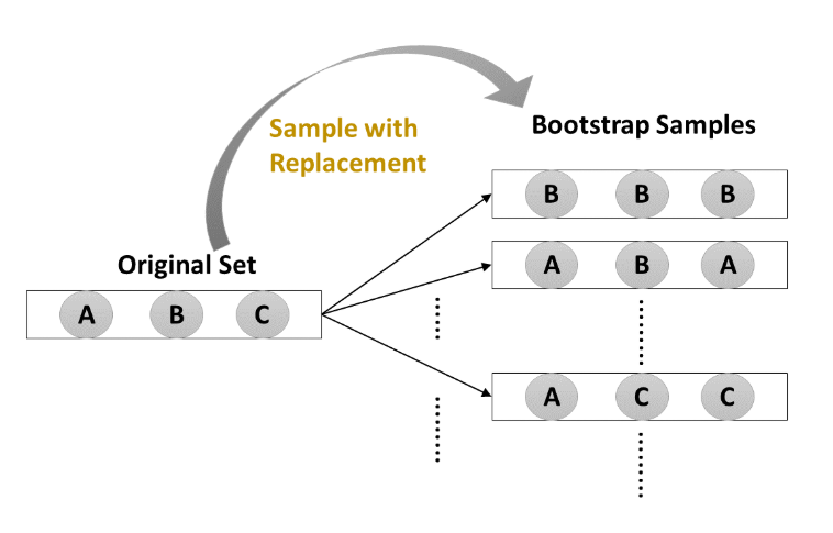
- Bootstrap Aggregation
- Uses a technique known as the bootstrap
- Reduces variance of individual models in the ensemble
_ Bootstrap
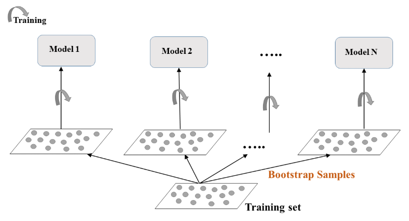
- Bootstrap-training
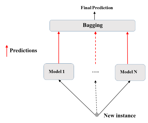
- Bootstrap-predict
Define the bagging classifier
In the following exercises you'll work with the Indian Liver Patient dataset from the UCI machine learning repository. Your task is to predict whether a patient suffers from a liver disease using 10 features including Albumin, age and gender. You'll do so using a Bagging Classifier.
- Preprocess
indian = pd.read_csv('./dataset/indian_liver_patient_preprocessed.csv', index_col=0)
indian.head()
| Age_std | Total_Bilirubin_std | Direct_Bilirubin_std | Alkaline_Phosphotase_std | Alamine_Aminotransferase_std | Aspartate_Aminotransferase_std | Total_Protiens_std | Albumin_std | Albumin_and_Globulin_Ratio_std | Is_male_std | Liver_disease | |
|---|---|---|---|---|---|---|---|---|---|---|---|
| 0 | 1.247403 | -0.420320 | -0.495414 | -0.428870 | -0.355832 | -0.319111 | 0.293722 | 0.203446 | -0.147390 | 0 | 1 |
| 1 | 1.062306 | 1.218936 | 1.423518 | 1.675083 | -0.093573 | -0.035962 | 0.939655 | 0.077462 | -0.648461 | 1 | 1 |
| 2 | 1.062306 | 0.640375 | 0.926017 | 0.816243 | -0.115428 | -0.146459 | 0.478274 | 0.203446 | -0.178707 | 1 | 1 |
| 3 | 0.815511 | -0.372106 | -0.388807 | -0.449416 | -0.366760 | -0.312205 | 0.293722 | 0.329431 | 0.165780 | 1 | 1 |
| 4 | 1.679294 | 0.093956 | 0.179766 | -0.395996 | -0.295731 | -0.177537 | 0.755102 | -0.930414 | -1.713237 | 1 | 1 |
X = indian.drop('Liver_disease', axis='columns')
y = indian['Liver_disease']
from sklearn.tree import DecisionTreeClassifier
from sklearn.ensemble import BaggingClassifier

# Instantiate dt
dt = DecisionTreeClassifier(random_state=1)

# Instantiate bc
bc = BaggingClassifier(base_estimator=dt, n_estimators=50, random_state=1)
Evaluate Bagging performance
Now that you instantiated the bagging classifier, it's time to train it and evaluate its test set accuracy.
from sklearn.model_selection import train_test_split

X_train, X_test, y_train, y_test = train_test_split(X, y, test_size=0.2, stratify=y, random_state=1)
from sklearn.metrics import accuracy_score

# Fit bc to the training set
bc.fit(X_train, y_train)

# Predict test set labels
y_pred = bc.predict(X_test)

# Evaluate acc_test
acc_test = accuracy_score(y_test, y_pred)
print('Test set accuracy of bc: {:.2f}'.format(acc_test))
Test set accuracy of bc: 0.71
dt.fit(X_train, y_train)

y_pred_dt = dt.predict(X_test)

acc_test_dt = accuracy_score(y_test, y_pred_dt)
print('Test set accuracy of dt: {:.2f}'.format(acc_test_dt))
Test set accuracy of dt: 0.63
Out of Bag Evaluation
- Bagging
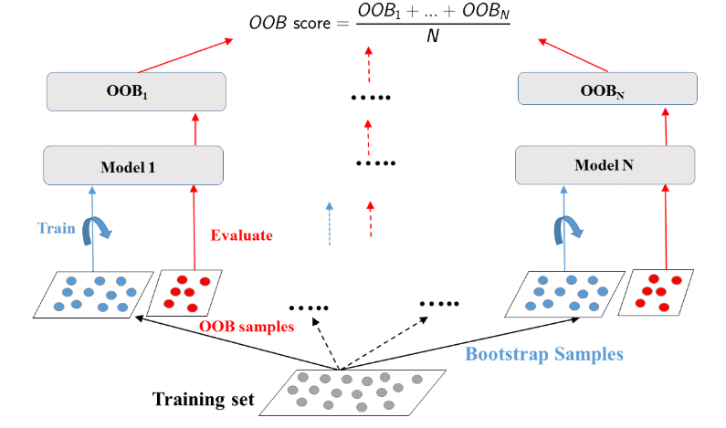
- Some instances may be sampled several times for one model, other instances may not be sampled at all.
- Out Of Bag (OOB) instances
- On average, for each model, 63% of the training instances are sampled
- The remaining 37% constitute the OOB instances
- OOB Evaluation
Prepare the ground
In the following exercises, you'll compare the OOB accuracy to the test set accuracy of a bagging classifier trained on the Indian Liver Patient dataset.
In sklearn, you can evaluate the OOB accuracy of an ensemble classifier by setting the parameter oob_score to True during instantiation. After training the classifier, the OOB accuracy can be obtained by accessing the .oob_score_ attribute from the corresponding instance.
from sklearn.tree import DecisionTreeClassifier
from sklearn.ensemble import BaggingClassifier

# Instantiate dt
dt = DecisionTreeClassifier(min_samples_leaf=8, random_state=1)

# Instantiate bc
bc = BaggingClassifier(base_estimator=dt, n_estimators=50, oob_score=True, random_state=1)
OOB Score vs Test Set Score
Now that you instantiated bc, you will fit it to the training set and evaluate its test set and OOB accuracies.
# Fit bc to the training set
bc.fit(X_train, y_train)

# Predict test set labels
y_pred = bc.predict(X_test)

# Evaluate test set accuracy
acc_test = accuracy_score(y_test, y_pred)

# Evaluate OOB accuracy
acc_oob = bc.oob_score_

# Print acc_test and acc_oob
print('Test set accuracy: {:.3f}, OOB accuracy: {:.3f}'.format(acc_test, acc_oob))
Test set accuracy: 0.698, OOB accuracy: 0.700
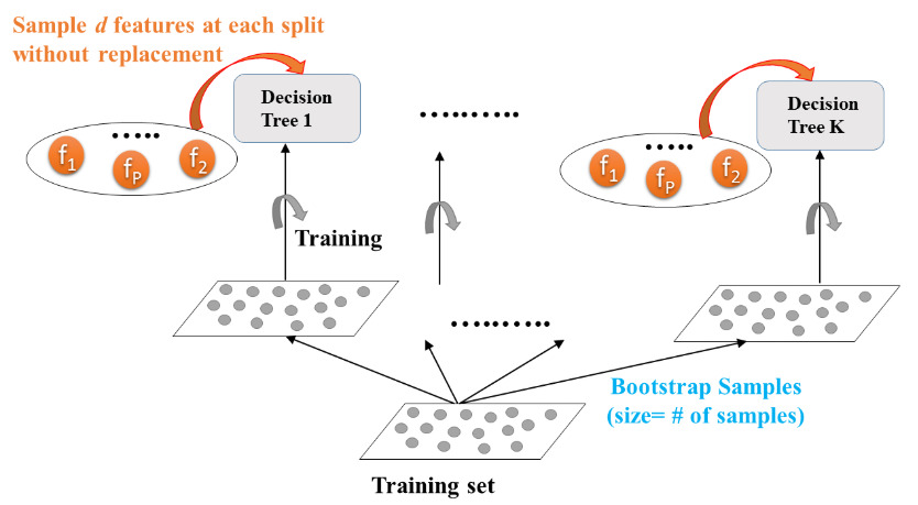
Random Forests (RF)
- Bagging
- Base estimator: Decision Tree, Logistic Regression, Neural Network, ...
- Each estimator is trained on a distinct bootstrap sample of the training set
- Estimators use all features for training and prediction
- Further Diversity with Random Forest
- Base estimator: Decision Tree
- Each estimator is trained on a different bootstrap sample having the same size as the training set
- RF introduces further randomization in the training of individual trees
- $d$ features are sampled at each node without replacement
- Random Forest: Training
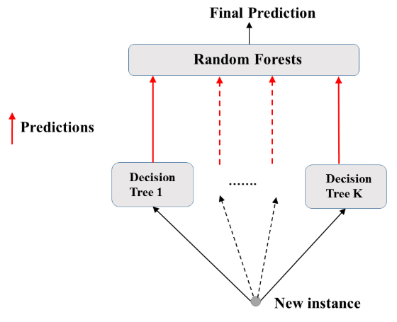
- Random Forest: Prediction
- Feature importance
- Tree based methods: enable measuring the importance of each feature in prediction
Train an RF regressor
In the following exercises you'll predict bike rental demand in the Capital Bikeshare program in Washington, D.C using historical weather data from the Bike Sharing Demand dataset available through Kaggle. For this purpose, you will be using the random forests algorithm. As a first step, you'll define a random forests regressor and fit it to the training set.
- Preprocess
bike = pd.read_csv('./dataset/bikes.csv')
bike.head()
| hr | holiday | workingday | temp | hum | windspeed | cnt | instant | mnth | yr | Clear to partly cloudy | Light Precipitation | Misty | |
|---|---|---|---|---|---|---|---|---|---|---|---|---|---|
| 0 | 0 | 0 | 0 | 0.76 | 0.66 | 0.0000 | 149 | 13004 | 7 | 1 | 1 | 0 | 0 |
| 1 | 1 | 0 | 0 | 0.74 | 0.70 | 0.1343 | 93 | 13005 | 7 | 1 | 1 | 0 | 0 |
| 2 | 2 | 0 | 0 | 0.72 | 0.74 | 0.0896 | 90 | 13006 | 7 | 1 | 1 | 0 | 0 |
| 3 | 3 | 0 | 0 | 0.72 | 0.84 | 0.1343 | 33 | 13007 | 7 | 1 | 1 | 0 | 0 |
| 4 | 4 | 0 | 0 | 0.70 | 0.79 | 0.1940 | 4 | 13008 | 7 | 1 | 1 | 0 | 0 |
X = bike.drop('cnt', axis='columns')
y = bike['cnt']
X_train, X_test, y_train, y_test = train_test_split(X, y, test_size=0.2, random_state=2)
from sklearn.ensemble import RandomForestRegressor

# Instantiate rf
rf = RandomForestRegressor(n_estimators=25, random_state=2)

# Fit rf to the training set
rf.fit(X_train, y_train)
RandomForestRegressor(bootstrap=True, ccp_alpha=0.0, criterion='mse',
                      max_depth=None, max_features='auto', max_leaf_nodes=None,
                      max_samples=None, min_impurity_decrease=0.0,
                      min_impurity_split=None, min_samples_leaf=1,
                      min_samples_split=2, min_weight_fraction_leaf=0.0,
                      n_estimators=25, n_jobs=None, oob_score=False,
                      random_state=2, verbose=0, warm_start=False)
Evaluate the RF regressor
You'll now evaluate the test set RMSE of the random forests regressor rf that you trained in the previous exercise.
from sklearn.metrics import mean_squared_error as MSE

# Predict the test set labels
y_pred = rf.predict(X_test)

# Evaluate the test set RMSE
rmse_test = MSE(y_test, y_pred) ** 0.5

# Print rmse_test
print('Test set RMSE of rf: {:.2f}'.format(rmse_test))
Test set RMSE of rf: 54.49
Visualizing features importances
In this exercise, you'll determine which features were the most predictive according to the random forests regressor rf that you trained in a previous exercise.
For this purpose, you'll draw a horizontal barplot of the feature importance as assessed by rf. Fortunately, this can be done easily thanks to plotting capabilities of pandas.
# Create a pd.Series of features importances
importances = pd.Series(data=rf.feature_importances_, index=X_train.columns)

# Sort importances
importances_sorted = importances.sort_values()

# Draw a horizontal barplot of importances_sorted
importances_sorted.plot(kind='barh', color='lightgreen')
plt.title('Features Importances')
plt.savefig('../images/feature_importances.png')

Apparently, hr and workingday are the most important features according to rf. The importances of these two features add up to more than 90%!