Regression in PySpark
Next you'll learn to create Linear Regression models. You'll also find out how to augment your data by engineering new predictors as well as a robust approach to selecting only the most relevant predictors. This is the Summary of lecture "Machine Learning with PySpark", via datacamp.
- toc: true
- badges: true
- comments: true
- author: Chanseok Kang
- categories: [Python, Datacamp, PySpark]
- image: images/bucketing.png
import pyspark
from pyspark.sql import SparkSession

import numpy as np
import pandas as pd
One-Hot Encoding
Encoding flight origin
The org column in the flights data is a categorical variable giving the airport from which a flight departs.
- ORD — O'Hare International Airport (Chicago)
- SFO — San Francisco International Airport
- JFK — John F Kennedy International Airport (New York)
- LGA — La Guardia Airport (New York)
- SMF — Sacramento
- SJC — San Jose
- TUS — Tucson International Airport
- OGG — Kahului (Hawaii)
Obviously this is only a small subset of airports. Nevertheless, since this is a categorical variable, it needs to be one-hot encoded before it can be used in a regression model.
spark = SparkSession.builder.master('local[*]').appName('flights').getOrCreate()

# Read data from CSV file
flights = spark.read.csv('./dataset/flights-larger.csv', sep=',', header=True, inferSchema=True,
                         nullValue='NA')

# Get number of records
print("The data contain %d records." % flights.count())

# View the first five records
flights.show(5)

# Check column data types
print(flights.printSchema())
print(flights.dtypes)
The data contain 275000 records.
+---+---+---+-------+------+---+----+------+--------+-----+
|mon|dom|dow|carrier|flight|org|mile|depart|duration|delay|
+---+---+---+-------+------+---+----+------+--------+-----+
| 10| 10|  1|     OO|  5836|ORD| 157|  8.18|      51|   27|
|  1|  4|  1|     OO|  5866|ORD| 466|  15.5|     102| null|
| 11| 22|  1|     OO|  6016|ORD| 738|  7.17|     127|  -19|
|  2| 14|  5|     B6|   199|JFK|2248| 21.17|     365|   60|
|  5| 25|  3|     WN|  1675|SJC| 386| 12.92|      85|   22|
+---+---+---+-------+------+---+----+------+--------+-----+
only showing top 5 rows

root
 |-- mon: integer (nullable = true)
 |-- dom: integer (nullable = true)
 |-- dow: integer (nullable = true)
 |-- carrier: string (nullable = true)
 |-- flight: integer (nullable = true)
 |-- org: string (nullable = true)
 |-- mile: integer (nullable = true)
 |-- depart: double (nullable = true)
 |-- duration: integer (nullable = true)
 |-- delay: integer (nullable = true)

None
[('mon', 'int'), ('dom', 'int'), ('dow', 'int'), ('carrier', 'string'), ('flight', 'int'), ('org', 'string'), ('mile', 'int'), ('depart', 'double'), ('duration', 'int'), ('delay', 'int')]
from pyspark.ml.feature import StringIndexer

flights = StringIndexer(inputCol='org', outputCol='org_idx').fit(flights).transform(flights)

flights.show()
+---+---+---+-------+------+---+----+------+--------+-----+-------+
|mon|dom|dow|carrier|flight|org|mile|depart|duration|delay|org_idx|
+---+---+---+-------+------+---+----+------+--------+-----+-------+
| 10| 10|  1|     OO|  5836|ORD| 157|  8.18|      51|   27|    0.0|
|  1|  4|  1|     OO|  5866|ORD| 466|  15.5|     102| null|    0.0|
| 11| 22|  1|     OO|  6016|ORD| 738|  7.17|     127|  -19|    0.0|
|  2| 14|  5|     B6|   199|JFK|2248| 21.17|     365|   60|    2.0|
|  5| 25|  3|     WN|  1675|SJC| 386| 12.92|      85|   22|    5.0|
|  3| 28|  1|     B6|   377|LGA|1076| 13.33|     182|   70|    3.0|
|  5| 28|  6|     B6|   904|ORD| 740|  9.58|     130|   47|    0.0|
|  1| 19|  2|     UA|   820|SFO| 679| 12.75|     123|  135|    1.0|
|  8|  5|  5|     US|  2175|LGA| 214|  13.0|      71|  -10|    3.0|
|  5| 27|  5|     AA|  1240|ORD|1197| 14.42|     195|  -11|    0.0|
|  8| 20|  6|     B6|   119|JFK|1182| 14.67|     198|   20|    2.0|
|  2|  3|  1|     AA|  1881|JFK|1090| 15.92|     200|   -9|    2.0|
|  8| 26|  5|     B6|    35|JFK|1028| 20.58|     193|  102|    2.0|
|  4|  9|  5|     AA|   336|ORD| 733|  20.5|     125|   32|    0.0|
|  3|  8|  2|     UA|   678|ORD| 733| 10.95|     129|   55|    0.0|
|  8| 10|  3|     OH|  6347|LGA| 292| 11.75|     102|    8|    3.0|
|  8| 14|  0|     UA|   624|ORD| 612| 17.92|     109|   57|    0.0|
|  4|  8|  4|     OH|  5585|JFK| 301| 13.25|      88|   23|    2.0|
|  1| 14|  4|     UA|  1524|SFO| 414| 14.87|      91|   27|    1.0|
|  1|  2|  6|     AA|  1341|ORD|1846|   7.5|     275|   26|    0.0|
+---+---+---+-------+------+---+----+------+--------+-----+-------+
only showing top 20 rows
Note:
OneHotEncoderEstimatoris replaced withOneHotEncoderin 3.0.0
from pyspark.ml.feature import OneHotEncoder

# Create an instance of the one hot encoder
onehot = OneHotEncoder(inputCols=['org_idx'], outputCols=['org_dummy'])

# Apply the one hot encoder to the flights data
onehot = onehot.fit(flights)
flights_onehot = onehot.transform(flights)

# Check the results
flights_onehot.select('org', 'org_idx', 'org_dummy').distinct().sort('org_idx').show()
+---+-------+-------------+
|org|org_idx|    org_dummy|
+---+-------+-------------+
|ORD|    0.0|(7,[0],[1.0])|
|SFO|    1.0|(7,[1],[1.0])|
|JFK|    2.0|(7,[2],[1.0])|
|LGA|    3.0|(7,[3],[1.0])|
|SMF|    4.0|(7,[4],[1.0])|
|SJC|    5.0|(7,[5],[1.0])|
|TUS|    6.0|(7,[6],[1.0])|
|OGG|    7.0|    (7,[],[])|
+---+-------+-------------+
Regression
Flight duration model - Just distance
In this exercise you'll build a regression model to predict flight duration (the duration column).
For the moment you'll keep the model simple, including only the distance of the flight (the km column) as a predictor.
flights_onehot.show(5)
+---+---+---+-------+------+---+----+------+--------+-----+-------+-------------+
|mon|dom|dow|carrier|flight|org|mile|depart|duration|delay|org_idx|    org_dummy|
+---+---+---+-------+------+---+----+------+--------+-----+-------+-------------+
| 10| 10|  1|     OO|  5836|ORD| 157|  8.18|      51|   27|    0.0|(7,[0],[1.0])|
|  1|  4|  1|     OO|  5866|ORD| 466|  15.5|     102| null|    0.0|(7,[0],[1.0])|
| 11| 22|  1|     OO|  6016|ORD| 738|  7.17|     127|  -19|    0.0|(7,[0],[1.0])|
|  2| 14|  5|     B6|   199|JFK|2248| 21.17|     365|   60|    2.0|(7,[2],[1.0])|
|  5| 25|  3|     WN|  1675|SJC| 386| 12.92|      85|   22|    5.0|(7,[5],[1.0])|
+---+---+---+-------+------+---+----+------+--------+-----+-------+-------------+
only showing top 5 rows
from pyspark.sql.functions import round

# Convert 'mile' to 'km' and drop 'mile' column
flights_onehot = flights_onehot.withColumn('km', round(flights_onehot.mile * 1.60934, 0)).drop('mile')

flights_onehot.show(5)
+---+---+---+-------+------+---+------+--------+-----+-------+-------------+------+
|mon|dom|dow|carrier|flight|org|depart|duration|delay|org_idx|    org_dummy|    km|
+---+---+---+-------+------+---+------+--------+-----+-------+-------------+------+
| 10| 10|  1|     OO|  5836|ORD|  8.18|      51|   27|    0.0|(7,[0],[1.0])| 253.0|
|  1|  4|  1|     OO|  5866|ORD|  15.5|     102| null|    0.0|(7,[0],[1.0])| 750.0|
| 11| 22|  1|     OO|  6016|ORD|  7.17|     127|  -19|    0.0|(7,[0],[1.0])|1188.0|
|  2| 14|  5|     B6|   199|JFK| 21.17|     365|   60|    2.0|(7,[2],[1.0])|3618.0|
|  5| 25|  3|     WN|  1675|SJC| 12.92|      85|   22|    5.0|(7,[5],[1.0])| 621.0|
+---+---+---+-------+------+---+------+--------+-----+-------+-------------+------+
only showing top 5 rows
from pyspark.ml.feature import VectorAssembler

# Create an assembler object
assembler = VectorAssembler(inputCols=['km'], outputCol='features')

# Consolidate predictor columns
flights = assembler.transform(flights_onehot)

flights.show(5)
+---+---+---+-------+------+---+------+--------+-----+-------+-------------+------+--------+
|mon|dom|dow|carrier|flight|org|depart|duration|delay|org_idx|    org_dummy|    km|features|
+---+---+---+-------+------+---+------+--------+-----+-------+-------------+------+--------+
| 10| 10|  1|     OO|  5836|ORD|  8.18|      51|   27|    0.0|(7,[0],[1.0])| 253.0| [253.0]|
|  1|  4|  1|     OO|  5866|ORD|  15.5|     102| null|    0.0|(7,[0],[1.0])| 750.0| [750.0]|
| 11| 22|  1|     OO|  6016|ORD|  7.17|     127|  -19|    0.0|(7,[0],[1.0])|1188.0|[1188.0]|
|  2| 14|  5|     B6|   199|JFK| 21.17|     365|   60|    2.0|(7,[2],[1.0])|3618.0|[3618.0]|
|  5| 25|  3|     WN|  1675|SJC| 12.92|      85|   22|    5.0|(7,[5],[1.0])| 621.0| [621.0]|
+---+---+---+-------+------+---+------+--------+-----+-------+-------------+------+--------+
only showing top 5 rows
flights_train, flights_test = flights.randomSplit([0.8, 0.2])
from pyspark.ml.regression import LinearRegression
from pyspark.ml.evaluation import RegressionEvaluator

# Create a regression object and train on training data
regression = LinearRegression(featuresCol='features', labelCol='duration').fit(flights_train)

# Create predictions for the test data and take a look at the predictions
predictions = regression.transform(flights_test)
predictions.select('duration', 'prediction').show(5, False)

# Calculate the RMSE
RegressionEvaluator(labelCol='duration', metricName='rmse').evaluate(predictions)
+--------+------------------+
|duration|prediction        |
+--------+------------------+
|420     |496.4735315834907 |
|379     |345.85941488647666|
|210     |222.65721887539473|
|164     |133.60633841501843|
|125     |133.60633841501843|
+--------+------------------+
only showing top 5 rows
17.27005980968751
Interpreting the coefficients
The linear regression model for flight duration as a function of distance takes the form
duration = $\alpha$ + $\beta$ × distance
where
- $\alpha$ — intercept (component of duration which does not depend on distance) and
- $\beta$ — coefficient (rate at which duration increases as a function of distance; also called the slope).
By looking at the coefficients of your model you will be able to infer
- how much of the average flight duration is actually spent on the ground and
- what the average speed is during a flight.
# Intercept (average minutes on ground)
inter = regression.intercept
print(inter)

# Coefficients
coefs = regression.coefficients
print(coefs)

# Average minutes per km
minutes_per_km = regression.coefficients[0]
print(minutes_per_km)

# Average speed in km per hour
avg_speed = 60 / minutes_per_km
print(avg_speed)
44.25256380341634
[0.07572353780644245]
0.07572353780644245
792.3560063103033
Flight duration model - Adding origin airport
Some airports are busier than others. Some airports are bigger than others too. Flights departing from large or busy airports are likely to spend more time taxiing or waiting for their takeoff slot. So it stands to reason that the duration of a flight might depend not only on the distance being covered but also the airport from which the flight departs.
You are going to make the regression model a little more sophisticated by including the departure airport as a predictor.
# Create an assembler object
assembler = VectorAssembler(inputCols=['km', 'org_dummy'], outputCol='features')

# Consolidate predictor columns
flights = assembler.transform(flights_onehot)

flights.show(5)
+---+---+---+-------+------+---+------+--------+-----+-------+-------------+------+--------------------+
|mon|dom|dow|carrier|flight|org|depart|duration|delay|org_idx|    org_dummy|    km|            features|
+---+---+---+-------+------+---+------+--------+-----+-------+-------------+------+--------------------+
| 10| 10|  1|     OO|  5836|ORD|  8.18|      51|   27|    0.0|(7,[0],[1.0])| 253.0|(8,[0,1],[253.0,1...|
|  1|  4|  1|     OO|  5866|ORD|  15.5|     102| null|    0.0|(7,[0],[1.0])| 750.0|(8,[0,1],[750.0,1...|
| 11| 22|  1|     OO|  6016|ORD|  7.17|     127|  -19|    0.0|(7,[0],[1.0])|1188.0|(8,[0,1],[1188.0,...|
|  2| 14|  5|     B6|   199|JFK| 21.17|     365|   60|    2.0|(7,[2],[1.0])|3618.0|(8,[0,3],[3618.0,...|
|  5| 25|  3|     WN|  1675|SJC| 12.92|      85|   22|    5.0|(7,[5],[1.0])| 621.0|(8,[0,6],[621.0,1...|
+---+---+---+-------+------+---+------+--------+-----+-------+-------------+------+--------------------+
only showing top 5 rows
flights_train, flights_test = flights.randomSplit([0.8, 0.2])

# Create a regression object and train on training data
regression = LinearRegression(featuresCol='features', labelCol='duration').fit(flights_train)

# Create predictions for the test data
predictions = regression.transform(flights_test)

# Calculate the RMSE on test data
RegressionEvaluator(labelCol='duration', metricName='rmse').evaluate(predictions)
11.068844362217451
Interpreting coefficients
Remember that origin airport, org, has eight possible values (ORD, SFO, JFK, LGA, SMF, SJC, TUS and OGG) which have been one-hot encoded to seven dummy variables in org_dummy.
The values for km and org_dummy have been assembled into features, which has eight columns with sparse representation. Column indices in features are as follows:
- 0 —
km - 1 —
ORD - 2 —
SFO - 3 —
JFK - 4 —
LGA - 5 —
SMF - 6 —
SJCand - 7 —
TUS.
Note that OGG does not appear in this list because it is the reference level for the origin airport category.
In this exercise you'll be using the intercept and coefficients attributes to interpret the model.
The coefficients attribute is a list, where the first element indicates how flight duration changes with flight distance.
# Average speed in km per hour
avg_speed_hour = 60 / regression.coefficients[0]
print(avg_speed_hour)

# Averate minutes on ground at OGG
inter = regression.intercept
print(inter)

# Average minutes on ground at JFK
avg_ground_jfk= inter + regression.coefficients[3]
print(avg_ground_jfk)

# Average minutes on ground at LGA
avg_ground_lga = inter + regression.coefficients[4]
print(avg_ground_lga)
807.3348263721097
16.056291454658716
68.7530254980533
62.839478468083115
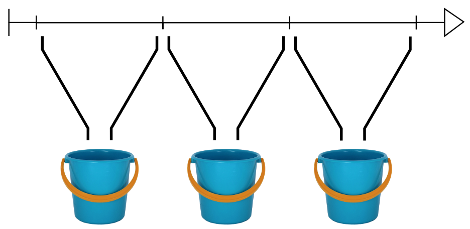
Bucketing departure time
Time of day data are a challenge with regression models. They are also a great candidate for bucketing.
In this lesson you will convert the flight departure times from numeric values between 0 (corresponding to "00:00") and 24 (corresponding to "24:00") to binned values. You'll then take those binned values and one-hot encode them.
from pyspark.ml.feature import Bucketizer

# Create buckets at 3 hour intervals through the day
buckets = Bucketizer(splits=[
    3 * x for x in range(9)
], inputCol='depart', outputCol='depart_bucket')

# Bucket the departure times
bucketed = buckets.transform(flights)
bucketed.select('depart', 'depart_bucket').show(5)

# Create a one-hot encoder
onehot = OneHotEncoder(inputCols=['depart_bucket'], outputCols=['depart_dummy'])

# One-hot encode the bucketed departure times
flights_onehot = onehot.fit(bucketed).transform(bucketed)
flights_onehot.select('depart', 'depart_bucket', 'depart_dummy').show(5)
+------+-------------+
|depart|depart_bucket|
+------+-------------+
|  8.18|          2.0|
|  15.5|          5.0|
|  7.17|          2.0|
| 21.17|          7.0|
| 12.92|          4.0|
+------+-------------+
only showing top 5 rows

+------+-------------+-------------+
|depart|depart_bucket| depart_dummy|
+------+-------------+-------------+
|  8.18|          2.0|(7,[2],[1.0])|
|  15.5|          5.0|(7,[5],[1.0])|
|  7.17|          2.0|(7,[2],[1.0])|
| 21.17|          7.0|    (7,[],[])|
| 12.92|          4.0|(7,[4],[1.0])|
+------+-------------+-------------+
only showing top 5 rows
Flight duration model - Adding departure time
In the previous exercise the departure time was bucketed and converted to dummy variables. Now you're going to include those dummy variables in a regression model for flight duration.
The data are in flights. The km, org_dummy and depart_dummy columns have been assembled into features, where km is index 0, org_dummy runs from index 1 to 7 and depart_dummy from index 8 to 14.
assembler = VectorAssembler(inputCols=['km', 'org_dummy', 'depart_dummy'], outputCol='features')

flights = assembler.transform(flights_onehot.drop('features'))

flights.show(5)
+---+---+---+-------+------+---+------+--------+-----+-------+-------------+------+-------------+-------------+--------------------+
|mon|dom|dow|carrier|flight|org|depart|duration|delay|org_idx|    org_dummy|    km|depart_bucket| depart_dummy|            features|
+---+---+---+-------+------+---+------+--------+-----+-------+-------------+------+-------------+-------------+--------------------+
| 10| 10|  1|     OO|  5836|ORD|  8.18|      51|   27|    0.0|(7,[0],[1.0])| 253.0|          2.0|(7,[2],[1.0])|(15,[0,1,10],[253...|
|  1|  4|  1|     OO|  5866|ORD|  15.5|     102| null|    0.0|(7,[0],[1.0])| 750.0|          5.0|(7,[5],[1.0])|(15,[0,1,13],[750...|
| 11| 22|  1|     OO|  6016|ORD|  7.17|     127|  -19|    0.0|(7,[0],[1.0])|1188.0|          2.0|(7,[2],[1.0])|(15,[0,1,10],[118...|
|  2| 14|  5|     B6|   199|JFK| 21.17|     365|   60|    2.0|(7,[2],[1.0])|3618.0|          7.0|    (7,[],[])|(15,[0,3],[3618.0...|
|  5| 25|  3|     WN|  1675|SJC| 12.92|      85|   22|    5.0|(7,[5],[1.0])| 621.0|          4.0|(7,[4],[1.0])|(15,[0,6,12],[621...|
+---+---+---+-------+------+---+------+--------+-----+-------+-------------+------+-------------+-------------+--------------------+
only showing top 5 rows
flights_train, flights_test = flights.randomSplit([0.8, 0.2])

# Train with training data
regression = LinearRegression(labelCol='duration').fit(flights_train)
predictions = regression.transform(flights_test)

RegressionEvaluator(labelCol='duration', metricName='rmse').evaluate(predictions)

# Average minutes on ground at OGG for flights departing between 21:00 and 24:00
avg_eve_ogg = regression.intercept
print(avg_eve_ogg)

# Average minutes on ground at OGG for flights departing between 00:00 and 03:00
avg_night_ogg = regression.intercept + regression.coefficients[8]
print(avg_night_ogg)

# Average minutes on ground at JFK for flights departing between 00:00 and 03:00
avg_night_jfk = regression.intercept + regression.coefficients[3] + regression.coefficients[8]
print(avg_night_jfk)
10.373606920439098
-4.299103533053989
47.724554377263395
Regularization
- Feature Selection
- Loss function
- Linear regression aims to minimize the MSE
- Loss function with regularization
- Add a regularization term which depends on coefficients
- Regularizer
    - Lasso - absolute value of the coefficients
    - Ridge - square of the coefficients
- Both will shrink the coefficients of unimportant predictors
- Strength of regularization determined by parameter $\lambda$:
    - $\lambda = 0$ - no regularization (standard regression)
    - $\lambda = \infty$ - complete regularization (all coefficients zero)
Flight duration model - More features!
Let's add more features to our model. This will not necessarily result in a better model. Adding some features might improve the model. Adding other features might make it worse.
More features will always make the model more complicated and difficult to interpret.
These are the features you'll include in the next model:
kmorg(origin airport, one-hot encoded, 8 levels)depart(departure time, binned in 3 hour intervals, one-hot encoded, 8 levels)dow(departure day of week, one-hot encoded, 7 levels) andmon(departure month, one-hot encoded, 12 levels).
These have been assembled into the features column, which is a sparse representation of 32 columns (remember one-hot encoding produces a number of columns which is one fewer than the number of levels).
onehot = OneHotEncoder(inputCols=['dow'], outputCols=['dow_dummy'])
flights = onehot.fit(flights).transform(flights)

onehot = OneHotEncoder(inputCols=['mon'], outputCols=['mon_dummy'])
flights = onehot.fit(flights).transform(flights)

flights.show(5)
+---+---+---+-------+------+---+------+--------+-----+-------+-------------+------+-------------+-------------+--------------------+-------------+---------------+
|mon|dom|dow|carrier|flight|org|depart|duration|delay|org_idx|    org_dummy|    km|depart_bucket| depart_dummy|            features|    dow_dummy|      mon_dummy|
+---+---+---+-------+------+---+------+--------+-----+-------+-------------+------+-------------+-------------+--------------------+-------------+---------------+
| 10| 10|  1|     OO|  5836|ORD|  8.18|      51|   27|    0.0|(7,[0],[1.0])| 253.0|          2.0|(7,[2],[1.0])|(15,[0,1,10],[253...|(6,[1],[1.0])|(11,[10],[1.0])|
|  1|  4|  1|     OO|  5866|ORD|  15.5|     102| null|    0.0|(7,[0],[1.0])| 750.0|          5.0|(7,[5],[1.0])|(15,[0,1,13],[750...|(6,[1],[1.0])| (11,[1],[1.0])|
| 11| 22|  1|     OO|  6016|ORD|  7.17|     127|  -19|    0.0|(7,[0],[1.0])|1188.0|          2.0|(7,[2],[1.0])|(15,[0,1,10],[118...|(6,[1],[1.0])|     (11,[],[])|
|  2| 14|  5|     B6|   199|JFK| 21.17|     365|   60|    2.0|(7,[2],[1.0])|3618.0|          7.0|    (7,[],[])|(15,[0,3],[3618.0...|(6,[5],[1.0])| (11,[2],[1.0])|
|  5| 25|  3|     WN|  1675|SJC| 12.92|      85|   22|    5.0|(7,[5],[1.0])| 621.0|          4.0|(7,[4],[1.0])|(15,[0,6,12],[621...|(6,[3],[1.0])| (11,[5],[1.0])|
+---+---+---+-------+------+---+------+--------+-----+-------+-------------+------+-------------+-------------+--------------------+-------------+---------------+
only showing top 5 rows
assembler = VectorAssembler(inputCols=[
    'km', 'org_dummy', 'depart_dummy', 'dow_dummy', 'mon_dummy'
], outputCol='features')

flights = assembler.transform(flights.drop('features'))
flights.show(5)
+---+---+---+-------+------+---+------+--------+-----+-------+-------------+------+-------------+-------------+-------------+---------------+--------------------+
|mon|dom|dow|carrier|flight|org|depart|duration|delay|org_idx|    org_dummy|    km|depart_bucket| depart_dummy|    dow_dummy|      mon_dummy|            features|
+---+---+---+-------+------+---+------+--------+-----+-------+-------------+------+-------------+-------------+-------------+---------------+--------------------+
| 10| 10|  1|     OO|  5836|ORD|  8.18|      51|   27|    0.0|(7,[0],[1.0])| 253.0|          2.0|(7,[2],[1.0])|(6,[1],[1.0])|(11,[10],[1.0])|(32,[0,1,10,16,31...|
|  1|  4|  1|     OO|  5866|ORD|  15.5|     102| null|    0.0|(7,[0],[1.0])| 750.0|          5.0|(7,[5],[1.0])|(6,[1],[1.0])| (11,[1],[1.0])|(32,[0,1,13,16,22...|
| 11| 22|  1|     OO|  6016|ORD|  7.17|     127|  -19|    0.0|(7,[0],[1.0])|1188.0|          2.0|(7,[2],[1.0])|(6,[1],[1.0])|     (11,[],[])|(32,[0,1,10,16],[...|
|  2| 14|  5|     B6|   199|JFK| 21.17|     365|   60|    2.0|(7,[2],[1.0])|3618.0|          7.0|    (7,[],[])|(6,[5],[1.0])| (11,[2],[1.0])|(32,[0,3,20,23],[...|
|  5| 25|  3|     WN|  1675|SJC| 12.92|      85|   22|    5.0|(7,[5],[1.0])| 621.0|          4.0|(7,[4],[1.0])|(6,[3],[1.0])| (11,[5],[1.0])|(32,[0,6,12,18,26...|
+---+---+---+-------+------+---+------+--------+-----+-------+-------------+------+-------------+-------------+-------------+---------------+--------------------+
only showing top 5 rows
flights_train, flights_test = flights.randomSplit([0.8, 0.2])

# Fit linear regressino model to training data
regression = LinearRegression(labelCol='duration').fit(flights_train)

# Make predictions on test data
predictions = regression.transform(flights_test)

# Calculate the RMSE on test data
rmse = RegressionEvaluator(labelCol='duration', metricName='rmse').evaluate(predictions)
print("The test RMSE is", rmse)

# Look at the model coefficients
coeffs = regression.coefficients
print(coeffs)
The test RMSE is 10.819088448211174
[0.07439903800595218,27.088541106962648,20.013200394243466,52.01818052724308,46.01830850977673,15.12491382457755,17.232738296408332,17.325183703296005,-14.71676008382402,-0.07217427091906863,4.005627327038735,7.010732946075667,4.716908120668705,8.858558301158828,8.985587137355129,-0.061725588783170936,-0.13593336494158573,-0.13496036395705654,-0.1433810465959523,-0.0442906254733511,-0.112404653935452,-1.8896756270865185,-1.8943555316508267,-1.9673036696221473,-3.395290942653575,-4.020286290569159,-3.830521589483759,-3.9812556715824035,-4.012225573392499,-3.8464412463732764,-2.630301804480476,-0.41142966468087394]
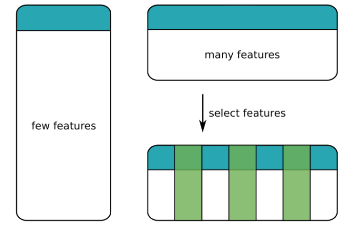
Flight duration model - Regularization!
In the previous exercise you added more predictors to the flight duration model. The model performed well on testing data, but with so many coefficients it was difficult to interpret.
In this exercise you'll use Lasso regression (regularized with a L1 penalty) to create a more parsimonious model. Many of the coefficients in the resulting model will be set to zero. This means that only a subset of the predictors actually contribute to the model. Despite the simpler model, it still produces a good RMSE on the testing data.
You'll use a specific value for the regularization strength. Later you'll learn how to find the best value using cross validation.
# Fit Lasso model (α = 1) to training data
regression = LinearRegression(labelCol='duration', regParam=1, elasticNetParam=1).fit(flights_train)
predictions = regression.transform(flights_test)

# Calculate the RMSE on testing data
rmse = RegressionEvaluator(labelCol='duration', metricName='rmse').evaluate(predictions)
print("The test RMSE is", rmse)

# Look at the model coefficients
coeffs = regression.coefficients
print(coeffs)

# Number of zero coefficients
zero_coeff = sum([beta == 0 for beta in regression.coefficients])
print("Number of coefficients equal to 0:", zero_coeff)
The test RMSE is 11.755155956333065
[0.07355997996294984,5.410341029649853,0.0,29.289003982755304,22.26237552623214,-2.1151843901573755,0.0,0.0,0.0,0.0,0.0,0.0,0.0,1.0987079734966165,1.3500916409600519,0.0,0.0,0.0,0.0,0.0,0.0,0.0,0.0,0.0,0.0,0.0,0.0,0.0,0.0,0.0,0.0,0.0]
Number of coefficients equal to 0: 25