import numpy as np
import matplotlib.pyplot as plt
import scipy.stats as sts
from celluloid import Camera
from IPython.display import HTML
import jax.numpy as jnp
import jax.scipy as jsc
from jax.nn import softmax

plt.rc("figure", figsize=(10.0, 3.0), dpi=120, facecolor="w")
np.random.seed(222)


def kde(x, data, h):
    return jnp.mean(jsc.stats.norm.pdf(x.reshape(-1, 1), loc=data, scale=h), axis=1)


def kde_hist(events, bins, bandwidth=None, density=False):
    """
    Args:
            events: (jax array-like) data to filter.

            bins: (jax array-like) intervals to calculate counts.

            bandwidth: (float) value that specifies the width of the individual
            distributions (kernels) whose cdfs are averaged over each bin. Defaults
            to Scott's rule -- the same as the scipy implementation of kde.

            density: (bool) whether or not to normalize the histogram to unit area.
    Returns:
            binned counts, calculated by kde!
    """
    bandwidth = bandwidth or events.shape[-1] ** -0.25  # Scott's rule

    edge_hi = bins[1:]  # ending bin edges ||<-
    edge_lo = bins[:-1]  # starting bin edges ->||

    # get cumulative counts (area under kde) for each set of bin edges
    cdf_up = jsc.stats.norm.cdf(edge_hi.reshape(-1, 1), loc=events, scale=bandwidth)
    cdf_dn = jsc.stats.norm.cdf(edge_lo.reshape(-1, 1), loc=events, scale=bandwidth)
    # sum kde contributions in each bin
    counts = (cdf_up - cdf_dn).sum(axis=1)

    if density:  # normalize by bin width and counts for total area = 1
        db = jnp.array(jnp.diff(bins), float)  # bin spacing
        return counts / db / counts.sum(axis=0)

    return counts
# This presentation is a Jupyter notebook! (thanks to https://github.com/damianavila/RISE )
2 * 2
4
Physics analysis as a differentiable program
Nathan Simpson
(supervised by & in collaboration with Lukas Heinrich)


We three things of presentation are:
What does it mean for analysis to be 'differentiable'?
- Why even care?
How can we differentiate physics?
- feat. smoothing, pyhf, autodiff
Seeing it in action: *neos*
- m a c h i n e l e a r n i n g!!!!! omg!!!!!!!

A typical analysis:
data → cutflow → observable → model → test statistic → hypothesis test → limits (p-values)

Free parameters: cut values, parameters of a multivariate observable
Can we optimize them?
Sure we can!
Here's what we might do:
- Cuts: grid search of cut positions
- Objective: maximize approximate median significance $Z_{A}^{\left(\sigma_{b}=0\right)}=\sqrt{2((s+b) \ln (1+s / b)-s)}$
- Observable (e.g. neural network): train parameters $\phi$ via gradient descent
- Objective: minimize binary cross entropy (signal vs background)
Why do the methods and objectives differ if they're in the same pipeline?
They don't have to!
- Sigmoid cut optimized wrt $Z_A$ using gradient descent: (notebook from Alex Held)
- Green curve is the cut profile, centered around the grey dotted line
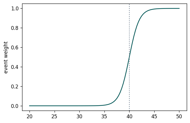
- Using $1/Z_A$ as a loss function: https://arxiv.org/abs/1806.00322
One could then imagine a jointly-optimized pipeline with respect to a single objective, trained using gradient descent.
This raises an important question:
- What should that objective be?
Picking the right objective
Insights from Sec 3.1, Deep Learning and its Application to LHC Physics:
"tools are often optimized for performance on a particular task that is several steps removed from the ultimate physical goal of searching for a new particle or testing a new
physical theory"
Picking the right objective
Insights from Sec 3.1, Deep Learning and its Application to LHC Physics:
"sensitivity to high-level physics questions must account for systematic uncertainties, which involve a nonlinear
trade-off between the typical machine learning performance metrics and the systematic uncertainty estimates."
We want:
- a goal that is directly related to our physics objective
- to take into account the full profile likelihood in order to be robust to systematic variations of nusiance parameters
But don't we already have this?

We can optimize our analysis end-to-end with respect to the actual significance... if we can evaluate its gradient.
Differentiable analysis:
Analysis with free parameters $\varphi$ that can be optimized end-to-end using gradient-based methods.
$$\varphi' = \varphi - \frac{\partial \, \mathsf{objective} }{\partial \, \mathsf{\varphi}}\times \mathsf{learning~rate} $$This is an example of differentiable programming, which is a superset of machine learning.
Due to the chain rule, every step in-between the objective and the parameters must also be differentiable.
e.g. $$\frac{\partial \, \mathsf{objective} }{\partial \, \mathsf{\varphi}} = \frac{\partial \, \mathsf{objective} }{\partial \, \mathsf{likelihood}} \times \frac{\partial \, \mathsf{likelihood} }{\partial \, \mathsf{model~parameters}}\times\frac{\partial \, \mathsf{model~parameters} }{\partial \, \mathsf{cut~values}}\times~...$$
... not guaranteed that all terms are finite, tractable, or even exist at all!
One could then imagine a jointly-optimized pipeline with respect to a single objective, trained using gradient descent.
This raises ~an~ two important questions:
- What should that objective be?
Can we evaluate its gradient?
- $\frac{\partial \, \mathsf{objective} }{\partial \, \mathsf{parameters}}$ = ?
- Is every step of the analysis differentiable?
Making physics differentiable: histograms
The height of the bins in a histogram do not vary smoothly with respect to shifts in the data. (remember, gradients are the language of small changes)
- But this is how optimizing analysis works -- updating the parameters (cuts, weights, etc.) changes the shape of the data downstream.
- We need that change to be well-behaved, as that's how we update the parameters in the first place!
fig = plt.figure()
cam = Camera(fig)
plt.xlim([-1, 4])
plt.axis("off")
bins = np.linspace(-1, 4, 7)
centers = bins[:-1] + np.diff(bins) / 2.0
grid = np.linspace(-1, 4, 500)
mu_range = np.linspace(1, 2, 100)
data = np.random.normal(size=100)
truths = sts.norm(loc=mu_range.reshape(-1, 1)).pdf(grid)
for i, mu in enumerate(mu_range):
    plt.plot(grid, truths[i], color="C1")  # plot true data distribution
    plt.hist(
        data + mu, bins=bins, density=True, color="C0", alpha=0.6
    )  # histogram data
    plt.axvline(mu, color="slategray", linestyle=":", alpha=0.6)
    cam.snap()
animation = cam.animate()
# HTML(animation.to_html5_video()) # uncomment for animation!

Making physics differentiable: histograms
An alternative: kernel density estimation
$$\mathsf{kde}(x ; h, \mathsf{data}) = \mathsf{mean}_{i\,\in\,\mathsf{len(data)}}\left[K\left(\frac{x-\mathsf{data}[i]}{h}\right)\right]\times \frac{1}{h}$$given some point $x$, kernel function $K$, and bandwith $h$ (smoothing parameter). In practice, the choice of $h$ has significantly more impact on the shape of the kde than the kernel choice.
Normally (ahem), we use the standard normal distribution for $K$
$$\Rightarrow \mathsf{kde}(x ; h) = \mathsf{mean}_{i\,\in\,\mathsf{len(data)}}[\mathsf{Normal}(\mu_i = \mathsf{data}[i], \sigma_i = h )(x)]$$This is just an average of gaussians centered at each data point! We control their widths globally using the bandwidth (one size fits all).
What happens when we vary the bandwidth?
Example for a 1-D gaussian:

If we want to estimate counts in a binned interval, we can still do that!
- The kde is just a mixture of gaussians, and has a tractable pdf/cdf
- For a bin with edges $[a,b]$, one can just evaluate the density $f(a\leqslant x<b)$

bw = 0.6
fig = plt.figure()
cam = Camera(fig)
plt.xlim([-1, 4])
plt.axis("off")
for i, mu in enumerate(mu_range):
    plt.plot(grid, truths[i], color="C1")
    plt.plot(grid, kde(grid, data + mu, h=bw), color="C9", linestyle=":")
    plt.bar(
        centers,
        kde_hist(data + mu, bins=bins, bandwidth=bw, density=True),
        color="C9",
        width=5 / (len(bins) - 1),
        alpha=0.6,
    )  # histogram data
    plt.axvline(mu, color="slategray", linestyle=":", alpha=0.6)
    cam.snap()
animation = cam.animate()
# animation.save('ani.gif',writer='imagemagick')
# HTML(animation.to_html5_video()) # uncomment for animation!
Another 'soft' histogram:
Could also use a softmax: $$ \mathsf{softmax}(\mathbf{x}; \tau)=\frac{e^{x_i / \tau}}{\sum_{i=0}^{\mathsf{len(\mathbf{x})}} e^{x_i / \tau}}$$
- $\tau$ is a softness hyperparameter, just like bandwidth!
- Softmax is a natural choice when working with a neural network that maps events to an observable
- $\mathbf{x}$ would be the output of $f$ for one event
- Then get normalized counts, with len(bins) = len(output of $f$)
Big thanks to the team :)
Making physics differentiable: profile likelihood ratio
Things get trickier when we consider the profile likelihood ratio:
$$\lambda(\mu)=\frac{L\left(\mu, \hat{\hat{\boldsymbol{\theta}}}\right)}{L\left(\hat{\mu}, \hat{\boldsymbol{\theta}}\right)}$$Both $\hat{\hat{\boldsymbol{\theta}}}$ and $(\hat{\boldsymbol{\theta}},\hat{\boldsymbol{\mu}})$ are defined by $\mathsf{argmax}$ operators, which involve doing maximum likelihood fits.
Fitting is not trivially differentiable!
Why not?
Normally involves a large number of iterations, which would be unrolled one-by-one when tracing computations
- We don't need all that information -- we just want to know how the final fitted values change!
The number of iterations doesn't vary smoothly
Solution? Fixed-point differentiation!
We can take advantage of the fact that $\mathsf{maximize}$ (or equivalently $\mathsf{minimize}$) routines have a fixed point:
- $\mathsf{minimize}$($L$, $x_{\mathsf{init}}$) = $x_*$
- $\mathsf{minimize}$($L$, $x_*$) = $x_*$
- $\Rightarrow\mathsf{minimize}(L,x_*)-x_*=0~~,$ so $x_*$ is a fixed point of $\mathsf{minimize}$.
Now that we know a fixed point exists, we can calculate the gradient using the converged iterations only!
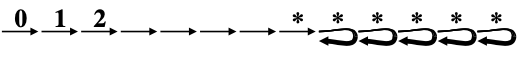
(graphic from this paper on adjoints of fixed-point iterations)
Which gradient, exactly?
The pyhf likelihood (and its local maxima) is implicitly a function of the signal and background yields. We need this gradient in the wider context of optimizing wrt the profile likelihood ratio:
$$\frac{\partial \, \mathsf{profile~likelihood} }{\partial \, \mathsf{\varphi}} = \frac{\partial \, \mathsf{profile~likelihood} }{\partial (s,b)} \times \frac{\partial (s,b)}{\partial \, \mathsf{\mathsf{\varphi}}}$$But then $\frac{\partial \, \mathsf{profile~likelihood} }{\partial (s,b)}$ involves $ \frac{\partial \, \mathsf{profile~likelihood} }{\partial \hat{\hat{\boldsymbol{\theta}}}} \times \frac{\partial \, \hat{\hat{\boldsymbol{\theta}}}}{\partial (s,b)}$ etc.
Think about the moving gaussian example: changing the parameter $\mu$ changed the shape of the histogram, but we don't write histogram(data,$\mu$). Likewise, we don't write $\hat{\hat{\boldsymbol{\theta}}}(s,b)$, but we can still find the gradient!
Putting it all together:
Recap:
- Using 'soft' histograms and cuts, we can differentiate computations up to the stage of constructing an observable.
- Thanks to pyhf, we have differentiable model building & likelihoods that build off of this observable.
- Combined with fixed-point differentiation, we can extend this differentiability downstream to the profile likelihood.
We now have the ingredients to differentiate a whole analysis!
Now comes the fun part: lets optimize it :)
Differentiable analysis in practice:

because we don't need a neural net for differentiable analysis (though we do use one :D)
Click me for Github! (and maybe leave a star... haha just kidding... unless?)

# Optional jax demo

neos demo: softmax, 2 bins, 2 background blobs
neos demo: kde, 3 bins, 3 background blobs (up/down variations)

Next steps:
A high-level roadmap:
- Actually release a paper (the software is citable though: https://zenodo.org/record/3697981#.Xw8KmJNKhhE)
- Make pyhf fully differentiable
- Would also be awesome to have awkward-array support autodiff (having this conversation on the side)
- More studies
- More differentiable tools
Next steps:
Many of these goals are the target of gradHEP!
gradHEP is an effort to consolidate differentiable building blocks for analysis into a set of common tools, and apply them.
See the 'Differentiable computing' HSF activity to find ways to get involved -- all are welcome at this very early stage! :)
Extra thanks:
- Pablo de Castro and Tommaso Dorigo for INFERNO (an inspiration for this work) and for discussions
- Folks in IRIS-HEP for their support & discussions
- Lukas for being a great supervisor
- The organisers of PyHEP! (you rock)
and thanks to you for listening!! :)
Twitters: @phi_nate, @lukasheinrich_
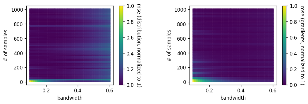
Backup: which bandwidth?
Can get an optimal bandwidth wrt 'mean integrated square error' if you do adaptive kdes: see this paper by Kyle Cranmer
Have also been doing some studies on bandwidth vs number of samples:
Backup: softmax v kde?
A future study to be done! See this issue on github
It's debatable whether you get any additional expressivity from putting a kde on top of a neural network (and in practice, it seems like the softmax converges more stably), but:
