BME 511 Fall 2021 Midterm Project: P300-based Brain Computer Interface¶

Assigned: October 06, 2021 Due: October 26, 2021

There is a dedicated channel for this project in the "Purdue BME511 Fall2021" Slack workspace. PDFs of the references cited here can be found in Brightspace.

Introduction¶

Brain-computer interfaces (BCIs) are an exciting possibility of modern-day Biomedical Engineering. They have a broad range of potential applications from augmenting human sensorimotor action in both medical (e.g., prostheses) and non-medical contexts (e.g., virtual-reality games), to neurofeedback for training and therapy (e.g., management of chronic pain, ADHD, rehabilitation after stroke). Electroencephalography (EEG) provides a non-invasive window to measure brain responses to various kinds of stimuli and how they interact with behaviors. In this project you will explore a classic BCI paradigm that uses EEG -- a P300 based on-screen menu selection. Classically, the P300 is a positive response peak that occurs in the EEG when an environmental stimulus happens to match a target expectation. It has been suggested that the P300 could be exploited to device a mental prosthetic that can be used for spelling when the patient is otherwise paralyzed (e.g., see Kübler et al., 2009).

In this project, you will use the data collected by Ulrich Hoffmann’s research group at EPFL accompanying their 2008 publication in the Journal of Neuroscience Methods (Hoffmann et al., 2008). Here, subjects were asked to concentrate on one of six different pictures on screen as they are periodically flashed one at a time and count the number of times the target flashed. The idea is that this simulates a scenario where a patient is trying to mentally select one of the six possible menu items on screen. When the target image (i.e., the one that the subject is concentrating on) flashes, the EEG data exhibits a P300 response (see Hoffmann et al., 2008 for details). The engineering problem is then one of decoding which of the six menu items the subject intended to select, by using just the EEG data. The faster the target is decoded from the EEG, the more quickly the action corresponding to the selected menu item can be executed. Further, the fewer the number of EEG channels required to decode the target, the interface becomes simpler and less intrusive. Also, if the features that differentiate the target menu item from the other items is consistent across multiple sessions for a given subjects, or is consistent across different individuals, then the BCI can be optimized for the “average” person without having to train the BCI for each individual or for each session. You will explore some of these issues in detail using signal processing techniques learnt in this course. For a broad discussion of EEG signal processing issues related to BCI, please see Lotte et al. (2014). However, note that Lotte et al. discuss some topics that we have not yet covered in class.

NOTE:

This “research” project represents a transition from the standard problem sets you have been doing to the independent research project you will do in the last 4-5 weeks of the course. This project is slightly more open-ended than the problem sets and asks more questions require analyzing/interpreting the results in the application-domain context. Thus, it is advised to take full advantage of the time allotted (~3 weeks, e.g., ~1 section per week, but remember that Part C is more open ended). Some readings from journal articles are provided so that you can further explore some of the issues that are surrounding this area of active interest both among engineers and neuroscientists. There are not necessarily right or wrong answers for some parts of this project. The point is to explore these signal-processing issues in a research-like manner. Note that some sections ask for research-like interpretations related to the field. Thus, a significant amount of the grading will be based on your ability to discuss the research implications of this work, not just getting the MATLAB/Python code to work. This emphasis is reflected in the point values for each section, which are provided at the end. Note, even if you can’t get some part of the code to work, you can (and should) still answer the research interpretation questions by assuming a certain outcome and providing a logical interpretation of what the implications would be if you had observed such an outcome.

Part A¶

Introduction to EEG preprocessing and extracting event-related brain responses. In this part, you will carry out a basic set of steps in EEG preprocessing to prepare the data for BCI use and to visually inspect for a P300 response. Simple visual inspection to get a sense for "what's in the data" is pretty much always the place to start for most signal processing problems. A description of the .mat files and the associated variables is given under the Dataset Description section, along with a download link.

1. Using Subject #6 (Control individual) as the example, develop MATLAB/Python functions to perform the following for each data file. Write your functions such that you can easily change which subject and session you are analyzing. In addition to signal processing experience, this part should also give you some basic practice for writing code to work with many different data files (e.g., using strings for file names etc.), which is useful in most data-science contexts.

   • For most electophysiological measurements, it is beneficial to have a reference channel (or few) on the body of the subject/patient (as opposed to just on the amplifier or power supply). Making a differential measurement of voltage this way can help reduce capacitive environmental noise because the reference channel will also pick up some of that noise. Re-reference data to the mastoid electrodes (Channels 33 and 34 are mastoid channels). That is, subtract from each channel’s data, the average between the mastoid channels (i.e., reference signal = 0.5 x signal in channel 33 + 0.5 x signal in channel 34; this reference signal is subtracted from the signals in each of the other channels).
   • Band-pass filter the data between 1 and 12 Hz using a relatively sharp FIR filter (say 0.5 Hz transition band). The standard recommendation made by EEG practitioners is to do filtering before the next step (segmenting to get “epochs”). Comment on why that may be so.
   • Extract single-trial responses (or “epochs”) for all non-target and target events by extracting the segment from time 0 to time 1000ms following each event. The events2samps() function given below would come in handy.
   • Subtract the “baseline” DC value from each trial. Here, the baseline DC value is the average value of the trial in the first 100 ms. This is so that slow drifts that are common in voltage measurements don't affect the individual trials. That is, after this step, each trial will swing around 0 rather than around some other constant value.
   • Reject noisy trials by checking if the data within that trial exceeds 40 microvolts (in either positive or negative directions). Note that the data are in microvolts to begin with, so the thresholding should be easy. Because of this step, your precise number of good trials might vary. This is primarily to remove movement related noise which is hard to remove (we'll see some wavelet-based denoising techniques later in the course that may help for problems like this).
   • Do not down-sample the data at this stage although done in Hoffman et al. Keep it at 2048 Hz. We can think about that in the dimensionality reduction step (Part C, subpart 4.).

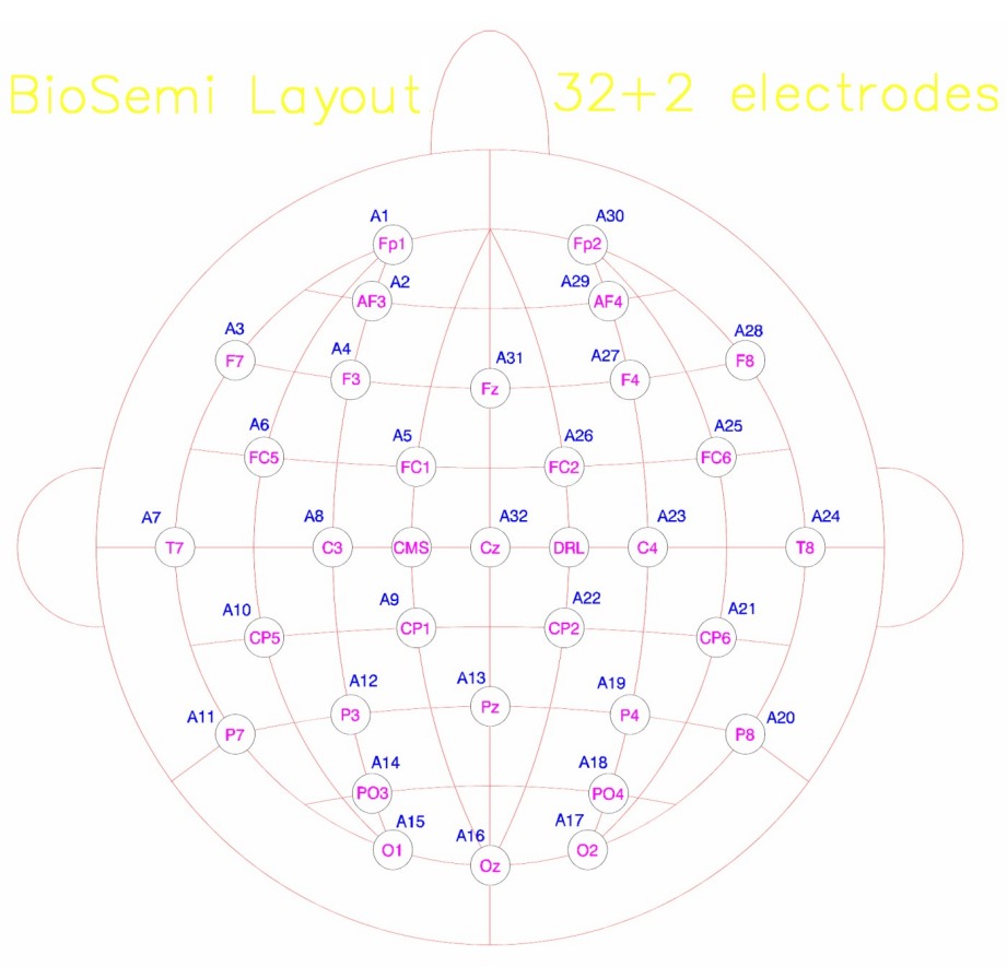
2. If you combine all files for any subject, you should get about 2500 non-target epochs and about 500 target epochs (your precise number of epochs will be different because of the epoch rejection). Average across all non-target epochs to get an averaged non-target response waveform. Similarly average across all target epochs across all sessions to get an averaged target response waveform. Plot the difference (target minus non-target) response with appropriate time axis. Do you see a P300 response for Subject 6? On which channels do you see them? Based on your results comment on which channels would be useful in discriminating target and non-target events. You can get a since of which channel number is where in the image below (mastoid electrodes not labeled here):

   

3. Repeat the process for at least one patient (choose arbitrarily; the paper gives you list of which subject numbers are controls and which are patients) for just channel Fz. Comment on how similar or not the results are across Subject 6 and the patient you chose, and what this means for your BCI application.

Part B¶

Extracting time-window of interest by statistical analysis on epoch data. In this part, you will use formal statistical analyses to determine which time segments differentiate target and non-target responses. Again, develop your analysis code with subject #6 as example to test and debug. Collapse across all files and sessions to get about 2500 non-target epochs and about 500 target epochs (your precise number of epochs will be different).

1. Assuming you have N non-target epochs, and M target epochs on a given channel (let’s start with just channel Fz), design a non-parametric test to see if the average difference response (average of M target epochs minus average of N non-target epochs) is distinguishable from noise. (Hint: If the null model is that the target and non-target responses are not different, then you can pool the (N+M) trials together into one basket and randomly break them into N and M epochs. Each such break can be used to get one null example. Thus you can generate examples of average difference responses you might see if the null model were in fact true.). Plot 100 null examples on top of the each other in grey/black color and then plot the actual difference between target and non-target trials in red and thicker line weight. For which continuous time window does the actual difference waveform standout as being different from the null examples (approximately)?

2. What is the p-value you get for channel Fz for subject #6, if you are using the positive peak height (max value) as the feature? For this calculation do at least 1000 null examples to get a more precise estimate.

3. Apply the statistical procedure to data from subject #6 for channels Cz, Pz, and Oz as well separately. What are the respective p-values for the peak height? Is the same time segment standing out (i.e., above your 1000 examples such that P < 0.001) for each of those channels? Identify this time segment manually and approximately (e.g., your answer could be something like “between XXX – YYY ms, the red trace stands out from the black traces/null examples”). Make note of this time interval for questions 4 and 5 in Part C.

Part C: Research considerations, and evaluating BCI potential¶

In this part, we will explore how much data we really need to see statistically discriminable P300 responses. Then we’ll formally evaluate BCI performance.

1. Continue with just Subject #6 and only focus on channel Fz. Now if you take only one session’s worth of data (Note that each subject has about 4 sessions, so we could think of this as taking just the first N/4 and M/4 trials respectively), what p-values do you get for the peak height? What if you reduced the number of trials to one file’s worth (each session has 6 files, so one file’s worth of data will be N/24 and M/24 trials respectively for non-target and target)? Comment on the significance of these observations for BCI.

2. How consistent are the results across files (i.e., across the twenty-four subdivisions each containing N/24 and M/24 trials respectively)? This can be quickly visualized by plotting the p-value for the peak of the P300 response across your 24 subdivisions. Comment on the significance of these observations for the real-world performance of the BCI.

3. Apply the same analyses on at least one patient (choose arbitrarily; the paper gives you list of which subject numbers are controls and which are patients). Based on your results, comment on how well you expect to perform for the patient if you "trained" your BCI using one file (i.e., 1/24th of the data) and "tested" it on the data from other files. Also comment on how your results for the patient’s data compare to that of subject #6 (which is a control subject).

4. Now let’s try to get a sense of what the BCI performance will be by designing a simple BCI by manual classification. Start with subject 6’s data again but keeping channels Fz, Cz, Pz and Oz. Collapse across all files and sessions to get about 2500 non-target epochs and about 500 target epochs (for each channel). In the real application, our goal is to take an arbitrary trial, extract information from that trial based on what you learnt from other/prior trials, and then see if you can correctly determine if the particular trial at hand is a “target” or “non-target” trial – In practical terms, you are trying to determine from the EEG response to a particular menu item whether the subject was mentally trying to select that menu-item or not. Each trial that you have will now correspond to four channels (Fz, Pz, Cz and Oz), and 1000 ms at the original sampling rate of 2048 Hz. That is, each waveform has a dimension of 4*2048 = 8192, which is too high to design a classifier (i.e., binary detector) by hand to separate target and non-target examples. Thus, choose a dimensionality reduction technique that will take you from 8192D to a small number (let's do 2D here). This could include down sampling (as in Hoffman et al., 2008), a priori selecting a time window of interest and throwing the rest, and PCA. During this process keep in mind the results from Part B, which helped identify which segments of time were important. Describe how you reduced the dimensionality of the data using precise language and the rationale for doing so. The sequence of steps you did to go from 8192 values per trial to two values per trial are an example of “feature extraction”.

Note:

In conventional signal processing, feature extraction is done based on an understanding of the underlying signal (like you are doing for this project). Modern machine learning techniques allow you both "learn" the features and classify them with minimal manual input (we'll see this later). However, the more modern approaches render the solution somewhat "black-box-y" and difficult to interpret, sometimes easily obscuring flaws in the design. Nonetheless, machine learning approaches can still be very powerful and useful when implemented with rigorous design principles and careful checks.

5. Plot the extracted features (one data point per trial) in the 2D space with different colors for target and non-target points. Are you able to manually design a classifier by choosing some boundaries (similar to how you did it with spike sorting in PS2) between the two clusters? It is unlikely that you will get clean separation with single trials. Repeat the plotting now with K=10 epochs averaged together, i.e., instead of classifying the (aproaximately) N = 2500, M=250 single trials, you should average trials 1:10, 11:20, 21:30, ... for non-target and target separately, and be left with (N/K) = 250 non-target averages and (M/K) = 25 target averages. Are you able to now draw a boundary? Explain what you see for K=10, 25, and 50.

6. Let’s say that the null hypothesis (H0) for the classifier is that a given trial is a "non-target" trial, and the alternate (H1) being that it is a “target” trial. When drawing broundaries between clusters, you can choose your boundaries to have more false alarms and fewer misses, or the other way around. Which way would you prefer and why? For the K=10 case from subpart 5, obtain and plot a rough ROC curve for target detection by choosing 8 different boundaries spanning a range of sensitivities and specificities. This ROC curve is a nice summary of the BCI performance for K=10. In terms of the real-world application of this BCI, what are some other ways in which you would want to evaluate its performance?

Points distribution (100 total, will be rescaled later to 20 points)

Part A (30 total)

1. 12
2. 8
3. 10

Part B (30 total)

1. 15
2. 10
3. 5

Part C (50 total)

1. 10
2. 5
3. 3
4. 12
5. 8
6. 12

References¶

Kübler, A., Furdea, A., Halder, S., Hammer, E. M., Nijboer, F., & Kotchoubey, B. (2009). A brain–computer interface controlled auditory event‐related potential (P300) spelling system for locked‐in patients. Annals of the New York Academy of Sciences, 1157(1), 90-100.

Hoffmann, U., Vesin, J. M., Ebrahimi, T., & Diserens, K. (2008). An efficient P300-based brain–computer interface for disabled subjects. Journal of Neuroscience methods, 167(1), 115-125.

Lotte, F. (2014). A tutorial on EEG signal-processing techniques for mental-state recognition in brain–computer interfaces. In Guide to Brain-Computer Music Interfacing (pp. 133-161). Springer London.

Dataset Description¶

These descriptions were kindly provided by Hoffman et al.

The data for this project can be downloaded from Dropbox here: https://www.dropbox.com/s/sjhomobqirk48i3/AllSubjsEEG.zip?dl=0

You will need a password to download the data. The password is available on Brightspace.

The data for all of the subjects is contained in the zip-archive AllSubjectsEEG.zip. Unpacking the archive should give you a folder for each subject (subject1, subject2, ... subject9). For subjectn, there will be four directories (subjectn/session1 to subjectn/session4). Each of the directories contains six .mat data files. Each file corresponds to one run (one sequence of flashes).

WARNING:

The data size is large (~2.2 GB). So download can take a while. If you are uploading this to your Google Drive for use with Colab, it will be enough to upload just the subjects you are choosing to analyze. That way, you can save space and better manage bandwidth constraints.

The following variables are contained in the data files:

• data:

This matrix contains the raw EEG. The dimension of the matrix is 34 × the number of samples. Each of the 34 rows corresponds to one electrode. The ordering of electrodes is: Fp1, AF3, F7, F3, FC1, FC5, T7, C3, CP1, CP5, P7, P3, Pz, PO3, O1, Oz, O2, PO4, P4, P8, CP6, CP2, C4, T8, FC6, FC2, F4, F8, AF4, Fp2, Fz, Cz, MA1, MA2. Each column corresponds to one temporal sample; the sampling rate is 2048 Hz. The data were recorded with a Biosemi Active Two system and not yet referenced to a channel on the body. Arbitrary referencing schemes can be implemented by subtracting the reference channel(s) from all other channels. In order to obtain a good signal-to-noise ratio it is highly recommended to always use referenced data (see also the FAQ section on the Biosemi homepage http://www.biosemi.com).

Hari's Note:

Please see step 1 in part A for instructions about suitable re-referencing steps for this project.

• events:

This matrix contains the time-points at which the flashes (events) occurred. In each of the datasets, the first flash comes 400 ms after the beginning of the EEG recording. To find the sample corresponding to the first flash, the sampling rate (2048 Hz) has to be multiplied by 0.4 (2048 × 0.4  = 820). To find the data samples corresponding to an arbitrary event E, the time of the first event has to be subtracted from the time of the event E. Then the time difference in seconds has to be multiplied by the sampling rate and the offset of 820 samples has to be added

Hari's Note:

This calculation to go from the events variable contained in the .mat files to a sequence of sample numbers is implemented by the events2samps() function below. You can just use this function instead of writing your own code, but you are encouraged to read through the code as an example of how to use datetime objects in python. The events2samps() function calls unpackStamp(), so you'll need to copy that too. Both of these functions need numpy imported as np and the datetime module. A MATLAB version of the function is also provided in case you are using MATLAB. The sequence of sample numbers (one number for each flash event) returned by this function can be used just like the sequence of sample numbers (one per click sound) were used for in the ABR newborn screening problem in PS2.

• stimuli:

This is an array containing the sequence of flashes. Entries have values between 1 and 6 and each entry corresponds to a flash of one image on the screen. The images on the screen are indexed as follows: 1) top left image, 2) top right image, 3) left image in the middle, etc. (see Figure 1 in Hoffman et al., 2008).

• target:

This variable contains the index of the image the user was focusing on. For example if target equals four, the user was counting the number of flashes of the image on the right in the middle.

• targets_counted:

This variable contains the number of flashes that were actually counted by the user. Together with the number of events this can be used to check if the user was really concentrated. For example if there are 120 events, the number of flashes that were actually counted should be 20.

MATLAB version of events2samps()¶

If you are using MATLAB, the function below implements the same function as the python code above.

function evesamps = events2samps(events, fs)

evesamps = zeros(1, size(events, 1));
for k = 1:size(events,1)
    evesamps(k) = round(etime(events(k, :), events(1, :))*fs...
        + 1 + 0.4*fs);
end