"데분방01) Basics and R environment"
"Basics and R environment"
- toc:true
- branch: master
- badges: true
- comments: true
- author: tingstyle1
- categories: [R, 통계, 대학원, 데분방1, R환경]
- image: "images/posts/data.png"
- 강의주소:https://lms.knou.ac.kr/dks/user/home/initUSTHomeIndex_GRSC.do?stLeftMenuId=0
- 선배블로그: https://insb.tistory.com/9?category=967351
- 작년 김성수 교수 강의로 진행
기본
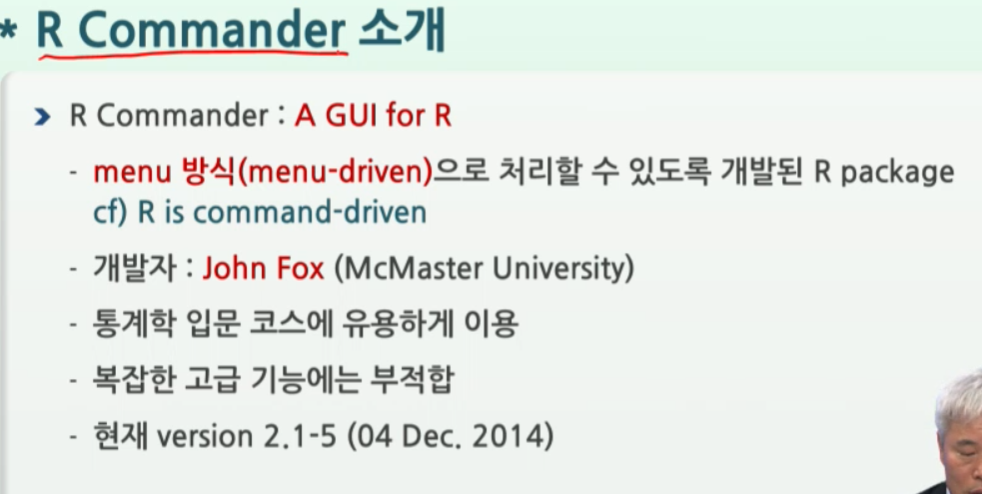
R 소개
- 무료
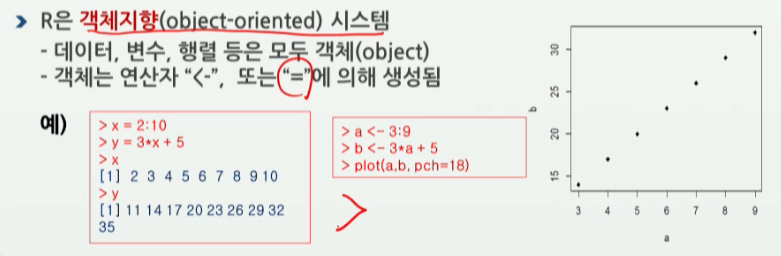
대화형프로그램 언어객체지향시스템- 데이터, 변수, 행렬 등은 모두 객체
- 생성은
=or<-로 생성
In [2]:
# 인덱싱이 다 inclusive네
x = 2:10
x
- 2
- 3
- 4
- 5
- 6
- 7
- 8
- 9
- 10
In [3]:
y <- 3*x + 5
y
- 11
- 14
- 17
- 20
- 23
- 26
- 29
- 32
- 35
In [4]:
a <- 3:9
b <- 3*a + 5
plot(a, b)

In [5]:
# pch는 point character -> 18번재의 pch(다이아먼드)로 그려라
plot(a, b, pch=18)

R의 역사
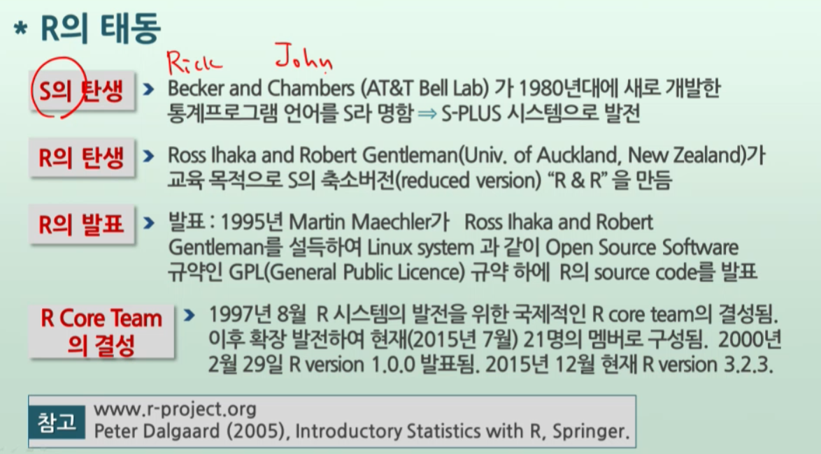
1980년대
S언어 탄생 by AT&T Bell Lab(c언어 개발한 연구소)에서 통계언어 S를 구현함- 1998 ACM S/W 상을 John Chambers가 탐 "Forever altered how people analyze, visualize and manipulate data
- 사람들이 어떻게 데이터 분석, 시각화, 다루는지를 영원히 바꾼 언어다
- 1998 ACM S/W 상을 John Chambers가 탐 "Forever altered how people analyze, visualize and manipulate data
오클란드 대학의 Ross and Robert 교수 2명이 S 축소버전인
R & R을 만듦1995년 Martin Maechler(마틴 매흘러)가 R&R(이하카, 젠틀만)을 설득하여, linux처럼 오픈소스(GPL)로 쓰게 한 것인
R source code발표1997년 8월
R core team결성. 2000년 02월 29일R version 1.0.0발표- 12월 R version 3.2.3
R 다운받기
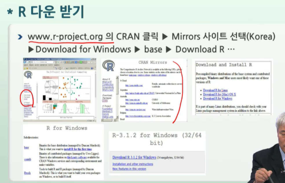
- base버전으로 다운 받기
작업영역 지정
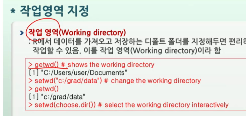
In [9]:
getwd()
'C:/Users/cho_desktop/2022_RProjects/대학원/1-01 데이터분석방법론 1'
In [8]:
# / 맥용 슬러쉬를 이용해서 절대경로 지정 c:/grad/data
setwd(".")
In [10]:
# 탐색기를 통해, 인터렉티브하게  직접 지정
setwd( choose.dir() )
Error in setwd(choose.dir()): missing value is invalid
Traceback:

1. setwd(choose.dir())
R studio 소개
- rsutdio.com
교재
First step
In [11]:
# ISwR 패키지 설치
install.packages("ISwR")
package 'ISwR' successfully unpacked and MD5 sums checked

The downloaded binary packages are in
	C:\Users\cho_desktop\AppData\Local\Temp\Rtmpo5uUeT\downloaded_packages
In [12]:
# 가동
library(ISwR)
Warning message:
"package 'ISwR' was built under R version 3.6.3"
In [13]:
# 정규분포를 따르는 r랜덤넘버 1000개
plot( rnorm(1000), pch = 19)

1.1.3 벡터연산
In [14]:
# 원소들끼리 순서대로 짝지어서 연산 가능한 장점 : 벡터연산c(,)의 장점
weight <- c(60, 72, 57, 90, 95, 72)
height <- c(1.75, 1.80, 1.65, 1.90, 1.74, 1.91)
bmi <- weight/height^2
In [15]:
bmi
- 19.5918367346939
- 22.2222222222222
- 20.9366391184573
- 24.9307479224377
- 31.3779891663364
- 19.7363010882377
In [16]:
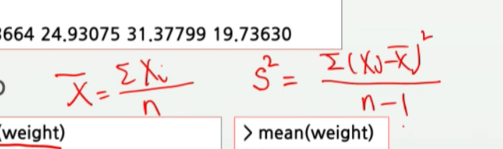
# 평균(xbar)과 SD 계산
# 벡터c의 갯수 -> length( )
xbar <- sum(weight) / length(weight)
xbar
74.3333333333333
In [17]:
mean(weight)
74.3333333333333
In [20]:
# sd: 편차 제곱의 n-1으로 나눈 평균
sqrt(sum((weight-xbar)^2) / (length(weight) - 1))
15.4229266569827
In [19]:
sd(weight)
15.4229266569827
1.1.4 standard procedures
In [21]:
bmi
- 19.5918367346939
- 22.2222222222222
- 20.9366391184573
- 24.9307479224377
- 31.3779891663364
- 19.7363010882377
In [22]:
# 1 표본 t검정(one sample t.test)
t.test(bmi, mu=22.5) # H0: mu=22.5 / H1: mu!=22.5

# t값 , 자유도, p값
	One Sample t-test

data:  bmi
t = 0.34488, df = 5, p-value = 0.7442
alternative hypothesis: true mean is not equal to 22.5
95 percent confidence interval:
 18.41734 27.84791
sample estimates:
mean of x
 23.13262
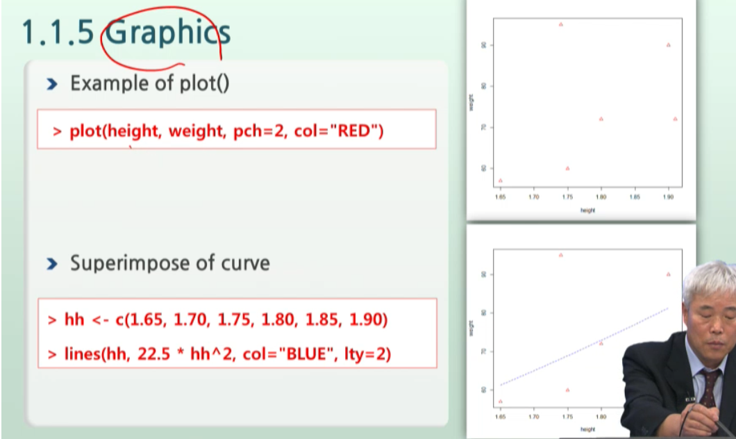
1.1.5 Graph
In [25]:
# 산점도

# color="대or소문자" 대신 col=2번호를 줘도 된다. like pch=숫자

plot(height, weight, pch=2, col="RED")

In [28]:
# R의 장점 -> 그림을 그리고 위에 덧그릴 수 있다. -> superimpose of curve


# c벡터객체 1개 만들고
hh <- c(1.65, 1.70, 1.75, 1.80, 1.85, 1.90)
# lines로 선 그리기
lines(hh, 22.5*hh^2, col="BLUE", lty=2) # lty = line type -> 2번은 점점점 타입
Error in plot.xy(xy.coords(x, y), type = type, ...): plot.new has not been called yet
Traceback:

1. lines(hh, 22.5 * hh^2, col = "BLUE", lty = 2)
2. lines.default(hh, 22.5 * hh^2, col = "BLUE", lty = 2)
3. plot.xy(xy.coords(x, y), type = type, ...)
In [29]:
# lines는 반드시 plot()그린 것 위에다 덧그리는 superimpose다.
plot(height, weight, pch=2, col="RED")

hh <- c(1.65, 1.70, 1.75, 1.80, 1.85, 1.90)
lines(hh, 22.5*hh^2, col="BLUE", lty=2)

1.2 R languange essentials
In [30]:
# 문자열 벡터는 큰/작은따옴표 다 쓸 수 있다.
# - 작따->큰따로 변환되서 표기된다.
# - 여기선 큰따-> 작따로 표기되네..like python
c("Huey", "Dewey", "Louie")
- 'Huey'
- 'Dewey'
- 'Louie'
In [31]:
c('Huey', 'Dewey', 'Louie')
- 'Huey'
- 'Dewey'
- 'Louie'
In [32]:
# True/False는   1글자로 정의-> 올 대문자로 표기된다.
c(T, T, F, T)
- TRUE
- TRUE
- FALSE
- TRUE
In [33]:
bmi
- 19.5918367346939
- 22.2222222222222
- 20.9366391184573
- 24.9307479224377
- 31.3779891663364
- 19.7363010882377
In [36]:
# logical vector
# 벡터 + 조건식 -> 마스크가 된다.
bmi > 25
- FALSE
- FALSE
- FALSE
- FALSE
- TRUE
- FALSE
In [37]:
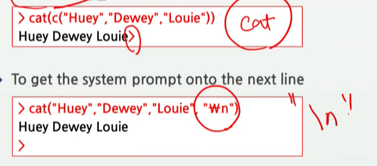
# 문자열 벡터를 1문자열로 연결 cat
cat( c("Huey", "Dewey", "Louie") )
Huey Dewey Louie
In [38]:
# 프롬프트에서 cat은 맨 뒤에 백슬래쉬n을 붙여 쓴다.
cat( c("Huey", "Dewey", "Louie", "\n") )
Huey Dewey Louie
In [39]:
# 특수문자ex>따옴표 도 사용하고 싶다면 backslash를 활요한다.
cat("What is \"R\"?\n")
What is "R"?
예제 참고자료 사이트
- 예제 파일을 들고 있는 블로그: https://booolean.tistory.com/913?category=807312
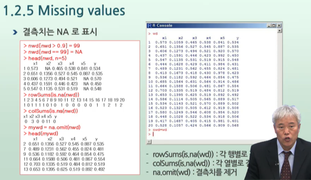
1.2.5 Missing Value
- R에서는 결측치를
NA로 표시한다.
In [45]:
# wd라는 데이터객체가 있다고 가정한다.
wd <- read.table("./data//01/wd.txt", sep = "\t", header=T) # "./따옴표경로" , sep="구분자" , header=T (첫줄이 타이틀)
wd
| M1 | M2 | M3 | M4 | M5 | Y |
|---|---|---|---|---|---|
| 0.573 | 0.1059 | 0.465 | 0.538 | 0.841 | 0.534 |
| 0.651 | 0.1356 | 0.527 | 0.545 | 0.887 | 0.535 |
| 0.606 | 0.1273 | 0.494 | 0.522 | 0.920 | 0.570 |
| 0.437 | 0.1591 | 0.446 | 0.423 | 0.992 | 0.450 |
| 0.547 | 0.1135 | 0.531 | 0.519 | 0.915 | 0.548 |
| 0.444 | 0.1628 | 0.429 | 0.411 | 0.984 | 0.431 |
| 0.489 | 0.1231 | 0.562 | 0.455 | 0.824 | 0.401 |
| 0.536 | 0.1473 | 0.410 | 0.430 | 0.978 | 0.423 |
| 0.413 | 0.1182 | 0.592 | 0.464 | 0.854 | 0.475 |
| 0.685 | 0.1564 | 0.631 | 0.564 | 0.914 | 0.486 |
| 0.664 | 0.1588 | 0.506 | 0.481 | 0.867 | 0.554 |
| 0.703 | 0.1335 | 0.519 | 0.484 | 0.812 | 0.519 |
| 0.653 | 0.1395 | 0.625 | 0.519 | 0.892 | 0.492 |
| 0.586 | 0.1114 | 0.505 | 0.565 | 0.889 | 0.517 |
| 0.534 | 0.1143 | 0.521 | 0.571 | 0.889 | 0.502 |
| 0.523 | 0.1320 | 0.508 | 0.412 | 0.919 | 0.508 |
| 0.580 | 0.1249 | 0.546 | 0.608 | 0.954 | 0.520 |
| 0.448 | 0.1028 | 0.522 | 0.534 | 0.918 | 0.506 |
| 0.417 | 0.1684 | 0.405 | 0.415 | 0.981 | 0.401 |
| 0.528 | 0.1057 | 0.424 | 0.566 | 0.909 | 0.568 |
In [46]:
# 객체를 = 할당으로 복사한다. (다른 언어에선 메모리주소 공유되서 안될 듯?)
nwd = wd

nwd
| M1 | M2 | M3 | M4 | M5 | Y |
|---|---|---|---|---|---|
| 0.573 | 0.1059 | 0.465 | 0.538 | 0.841 | 0.534 |
| 0.651 | 0.1356 | 0.527 | 0.545 | 0.887 | 0.535 |
| 0.606 | 0.1273 | 0.494 | 0.522 | 0.920 | 0.570 |
| 0.437 | 0.1591 | 0.446 | 0.423 | 0.992 | 0.450 |
| 0.547 | 0.1135 | 0.531 | 0.519 | 0.915 | 0.548 |
| 0.444 | 0.1628 | 0.429 | 0.411 | 0.984 | 0.431 |
| 0.489 | 0.1231 | 0.562 | 0.455 | 0.824 | 0.401 |
| 0.536 | 0.1473 | 0.410 | 0.430 | 0.978 | 0.423 |
| 0.413 | 0.1182 | 0.592 | 0.464 | 0.854 | 0.475 |
| 0.685 | 0.1564 | 0.631 | 0.564 | 0.914 | 0.486 |
| 0.664 | 0.1588 | 0.506 | 0.481 | 0.867 | 0.554 |
| 0.703 | 0.1335 | 0.519 | 0.484 | 0.812 | 0.519 |
| 0.653 | 0.1395 | 0.625 | 0.519 | 0.892 | 0.492 |
| 0.586 | 0.1114 | 0.505 | 0.565 | 0.889 | 0.517 |
| 0.534 | 0.1143 | 0.521 | 0.571 | 0.889 | 0.502 |
| 0.523 | 0.1320 | 0.508 | 0.412 | 0.919 | 0.508 |
| 0.580 | 0.1249 | 0.546 | 0.608 | 0.954 | 0.520 |
| 0.448 | 0.1028 | 0.522 | 0.534 | 0.918 | 0.506 |
| 0.417 | 0.1684 | 0.405 | 0.415 | 0.981 | 0.401 |
| 0.528 | 0.1057 | 0.424 | 0.566 | 0.909 | 0.568 |
In [47]:
# 0.9보다 큰 것만 골라서 99로 바꿔보자.
nwd[ nwd > 0.9 ] = 99
In [51]:
head(nwd)
| M1 | M2 | M3 | M4 | M5 | Y |
|---|---|---|---|---|---|
| 0.573 | 0.1059 | 0.465 | 0.538 | 0.841 | 0.534 |
| 0.651 | 0.1356 | 0.527 | 0.545 | 0.887 | 0.535 |
| 0.606 | 0.1273 | 0.494 | 0.522 | 99.000 | 0.570 |
| 0.437 | 0.1591 | 0.446 | 0.423 | 99.000 | 0.450 |
| 0.547 | 0.1135 | 0.531 | 0.519 | 99.000 | 0.548 |
| 0.444 | 0.1628 | 0.429 | 0.411 | 99.000 | 0.431 |
In [52]:
# 0.9보다 큰 99를 다시 NA로 바꿔보자.
nwd[nwd == 99] = NA

head(nwd)
| M1 | M2 | M3 | M4 | M5 | Y |
|---|---|---|---|---|---|
| 0.573 | 0.1059 | 0.465 | 0.538 | 0.841 | 0.534 |
| 0.651 | 0.1356 | 0.527 | 0.545 | 0.887 | 0.535 |
| 0.606 | 0.1273 | 0.494 | 0.522 | NA | 0.570 |
| 0.437 | 0.1591 | 0.446 | 0.423 | NA | 0.450 |
| 0.547 | 0.1135 | 0.531 | 0.519 | NA | 0.548 |
| 0.444 | 0.1628 | 0.429 | 0.411 | NA | 0.431 |
In [53]:
# 행별 결측치 : 결측치마스크 + 행별 합

# is.na()는 데이터객체 전체에 대한 boolean mask(logical character)를 만든다. -> 행렬mask -> 행 or 열별로 접근해줘야한다.
is.na(nwd)
| M1 | M2 | M3 | M4 | M5 | Y |
|---|---|---|---|---|---|
| FALSE | FALSE | FALSE | FALSE | FALSE | FALSE |
| FALSE | FALSE | FALSE | FALSE | FALSE | FALSE |
| FALSE | FALSE | FALSE | FALSE | TRUE | FALSE |
| FALSE | FALSE | FALSE | FALSE | TRUE | FALSE |
| FALSE | FALSE | FALSE | FALSE | TRUE | FALSE |
| FALSE | FALSE | FALSE | FALSE | TRUE | FALSE |
| FALSE | FALSE | FALSE | FALSE | FALSE | FALSE |
| FALSE | FALSE | FALSE | FALSE | TRUE | FALSE |
| FALSE | FALSE | FALSE | FALSE | FALSE | FALSE |
| FALSE | FALSE | FALSE | FALSE | TRUE | FALSE |
| FALSE | FALSE | FALSE | FALSE | FALSE | FALSE |
| FALSE | FALSE | FALSE | FALSE | FALSE | FALSE |
| FALSE | FALSE | FALSE | FALSE | FALSE | FALSE |
| FALSE | FALSE | FALSE | FALSE | FALSE | FALSE |
| FALSE | FALSE | FALSE | FALSE | FALSE | FALSE |
| FALSE | FALSE | FALSE | FALSE | TRUE | FALSE |
| FALSE | FALSE | FALSE | FALSE | TRUE | FALSE |
| FALSE | FALSE | FALSE | FALSE | TRUE | FALSE |
| FALSE | FALSE | FALSE | FALSE | TRUE | FALSE |
| FALSE | FALSE | FALSE | FALSE | TRUE | FALSE |
In [54]:
rowSums( is.na(nwd) )
- 0
- 0
- 1
- 1
- 1
- 1
- 0
- 1
- 0
- 1
- 0
- 0
- 0
- 0
- 0
- 1
- 1
- 1
- 1
- 1
In [55]:
colSums( is.na(nwd) )
- M1
- 0
- M2
- 0
- M3
- 0
- M4
- 0
- M5
- 11
- Y
- 0
In [56]:
# NA를 제거한 데이터를 복사할 수 있다.
# -> 행별로 제거하는 듯 싶다.
# -> na.omit()의 결과 <기존 행번호>가 같이 찍히니 확인하면 된다.
na.omit(nwd)
| M1 | M2 | M3 | M4 | M5 | Y | |
|---|---|---|---|---|---|---|
| 1 | 0.573 | 0.1059 | 0.465 | 0.538 | 0.841 | 0.534 |
| 2 | 0.651 | 0.1356 | 0.527 | 0.545 | 0.887 | 0.535 |
| 7 | 0.489 | 0.1231 | 0.562 | 0.455 | 0.824 | 0.401 |
| 9 | 0.413 | 0.1182 | 0.592 | 0.464 | 0.854 | 0.475 |
| 11 | 0.664 | 0.1588 | 0.506 | 0.481 | 0.867 | 0.554 |
| 12 | 0.703 | 0.1335 | 0.519 | 0.484 | 0.812 | 0.519 |
| 13 | 0.653 | 0.1395 | 0.625 | 0.519 | 0.892 | 0.492 |
| 14 | 0.586 | 0.1114 | 0.505 | 0.565 | 0.889 | 0.517 |
| 15 | 0.534 | 0.1143 | 0.521 | 0.571 | 0.889 | 0.502 |
In [57]:
nwd
| M1 | M2 | M3 | M4 | M5 | Y |
|---|---|---|---|---|---|
| 0.573 | 0.1059 | 0.465 | 0.538 | 0.841 | 0.534 |
| 0.651 | 0.1356 | 0.527 | 0.545 | 0.887 | 0.535 |
| 0.606 | 0.1273 | 0.494 | 0.522 | NA | 0.570 |
| 0.437 | 0.1591 | 0.446 | 0.423 | NA | 0.450 |
| 0.547 | 0.1135 | 0.531 | 0.519 | NA | 0.548 |
| 0.444 | 0.1628 | 0.429 | 0.411 | NA | 0.431 |
| 0.489 | 0.1231 | 0.562 | 0.455 | 0.824 | 0.401 |
| 0.536 | 0.1473 | 0.410 | 0.430 | NA | 0.423 |
| 0.413 | 0.1182 | 0.592 | 0.464 | 0.854 | 0.475 |
| 0.685 | 0.1564 | 0.631 | 0.564 | NA | 0.486 |
| 0.664 | 0.1588 | 0.506 | 0.481 | 0.867 | 0.554 |
| 0.703 | 0.1335 | 0.519 | 0.484 | 0.812 | 0.519 |
| 0.653 | 0.1395 | 0.625 | 0.519 | 0.892 | 0.492 |
| 0.586 | 0.1114 | 0.505 | 0.565 | 0.889 | 0.517 |
| 0.534 | 0.1143 | 0.521 | 0.571 | 0.889 | 0.502 |
| 0.523 | 0.1320 | 0.508 | 0.412 | NA | 0.508 |
| 0.580 | 0.1249 | 0.546 | 0.608 | NA | 0.520 |
| 0.448 | 0.1028 | 0.522 | 0.534 | NA | 0.506 |
| 0.417 | 0.1684 | 0.405 | 0.415 | NA | 0.401 |
| 0.528 | 0.1057 | 0.424 | 0.566 | NA | 0.568 |
1.2.6 Functions that create vectors
In [59]:
# 벡터생성은 create의 c()로 각 객체들을 연결해서 벡터를 만든다.
x <- c(1,2,3)
y <- c(10, 20)

c(x, y, 5) # 벡터객체와 값이 동등하게 1차원으로 연결된다.
- 1
- 2
- 3
- 10
- 20
- 5
In [62]:
# 다양한 타입이 벡터안의 요소로 들어갈 경우, 제한적인 쪽으로 자동 convert된다.

# boolean + 숫자 -> 숫자로 type 0/1로 바뀌어서 type통일
c(FALSE, 3)
- 0
- 3
In [63]:
# boolean + 문자열 -> 문자열로 바뀐다.
c(FALSE, "abc")
- 'FALSE'
- 'abc'
In [64]:
# 상수+ 문자열 -> 문자열
c(pi, "abc")
- '3.14159265358979'
- 'abc'
In [65]:
# 연속적인 값은 한번에 벡터로 생성할 수 있다.
seq(4, 9)
- 4
- 5
- 6
- 7
- 8
- 9
In [66]:
oops <- c(7, 9, 13)
In [68]:
# 반복문대신 단순 [원소복사] 반복 해주는 rep
rep(oops, 3)
- 7
- 9
- 13
- 7
- 9
- 13
- 7
- 9
- 13
In [78]:
# 반복을 원소위치에 따라 지정해줄 수 도 있다.
# - index순서대로 1번, 2번, 3번 반복복사
# - index별 반복회수도 벡터로 제공하면 된다.
rep(oops, c(1,2,3))
- 7
- 9
- 9
- 13
- 13
- 13
In [79]:
rep(oops, 1:3)
- 7
- 9
- 9
- 13
- 13
- 13
In [80]:
# 벡터1과 2가 있고, 1을 10번, 2을 15번
rep(1:2, c(10, 15))
- 1
- 1
- 1
- 1
- 1
- 1
- 1
- 1
- 1
- 1
- 2
- 2
- 2
- 2
- 2
- 2
- 2
- 2
- 2
- 2
- 2
- 2
- 2
- 2
- 2
1.2.7 Matrices and arrays
In [81]:
x <- 1:12
x
- 1
- 2
- 3
- 4
- 5
- 6
- 7
- 8
- 9
- 10
- 11
- 12
In [84]:
# 1차원 벡터에 대해, 차원을 c(3, 4) 벡터로 만들어서 dim()에 넣어주면
# 행렬이 된다.
dim(x) = c(3, 4)

x # 보이진 않지만, 1, 2, 3, 행    ,1 ,2 ,3 ,4 렬이 된다.
| 1 | 4 | 7 | 10 |
| 2 | 5 | 8 | 11 |
| 3 | 6 | 9 | 12 |
In [85]:
# 애초에 생성할 떄부터 m,n차원 matrix를 만들 수 도 있다.
# - 특히 byrow=를 T루로 주면, ncol없이 알아서 된다.
matrix(1:12, nrow=3, byrow=T)
| 1 | 2 | 3 | 4 |
| 5 | 6 | 7 | 8 |
| 9 | 10 | 11 | 12 |
In [ ]:
In [86]:
LETTERS[1:3]
- 'A'
- 'B'
- 'C'
In [87]:
# 행렬의 row에 rownames를 걸어줄 수 있다.
rownames(x) <- LETTERS[1:3]
In [88]:
x
| A | 1 | 4 | 7 | 10 |
|---|---|---|---|---|
| B | 2 | 5 | 8 | 11 |
| C | 3 | 6 | 9 | 12 |
In [89]:
# transverse는 t()로 하면 된다.
t(x)
| A | B | C |
|---|---|---|
| 1 | 2 | 3 |
| 4 | 5 | 6 |
| 7 | 8 | 9 |
| 10 | 11 | 12 |
In [91]:
# 1차원들을 -> 세워서 열로 합하는 cbind
# 1차원들을 -> 눕혀서 행으로 더하는 rbind

cbind(A = 1:4)
| A |
|---|
| 1 |
| 2 |
| 3 |
| 4 |
In [92]:
cbind(A = 1:4, B = 5:6, C = 9:12)
| A | B | C |
|---|---|---|
| 1 | 5 | 9 |
| 2 | 6 | 10 |
| 3 | 5 | 11 |
| 4 | 6 | 12 |
In [93]:
rbind(A=1:4,B=5:8,C=9:12)
| A | 1 | 2 | 3 | 4 |
|---|---|---|---|---|
| B | 5 | 6 | 7 | 8 |
| C | 9 | 10 | 11 | 12 |
In [95]:
aa <- cbind(A=1:4,B=5:8,C=9:12)
aa
| A | B | C |
|---|---|---|
| 1 | 5 | 9 |
| 2 | 6 | 10 |
| 3 | 7 | 11 |
| 4 | 8 | 12 |
In [97]:
# bind에서 상수를 넣으면, 방향 전체가 1로 채워진다.
# - 좌or우 똑같은 크기의 상수를 붙이려면 상수로 bind하면 된다.

cbind(1, aa)
| A | B | C | |
|---|---|---|---|
| 1 | 1 | 5 | 9 |
| 1 | 2 | 6 | 10 |
| 1 | 3 | 7 | 11 |
| 1 | 4 | 8 | 12 |
factors(범주형 자료)
카테고리칼 변수는인자로 만들어주는게 중요하다. 그 때 쓰는 것이factor()
In [98]:
pain <- c(0, 3, 2, 2, 1)
In [99]:
# 앞에 f를 붙여 factor임을 명시해주자.
# -> levels=에는 [요인들과 동일한 값]으로 레벨을 정해서 매칭해놓는다.
# -> 연속적인 숫자벡터를 줬어도 '0'~'3'의 문자열로 정해진다.
# -> 매칭된 요인-레벨에 대해서, 레벨이름levels을 바꿔주면 요인들도 따라 바뀐다.

fpain <- factor(pain, levels = 0:3)

fpain
- 0
- 3
- 2
- 2
- 1
Levels:
- '0'
- '1'
- '2'
- '3'
In [102]:
# factor의 [levels의 이름]을 문자열 벡터로 level에 대한 [라벨]적용이 가능하다.
# -> 원본 값들이 레벨에 따른 해당 [라벨]로 바껴버린다.
levels(fpain) <- c("none", "mild", "medium", "severe")

fpain
- none
- severe
- medium
- medium
- mild
Levels:
- 'none'
- 'mild'
- 'medium'
- 'severe'
숫자 -> 라벨 by요인덮 바꾸기

변수 job, edu를 숫자 -> 라벨(요인)으로 바꿔보자.
In [130]:
insurance = read.table("./data/01//insurance.txt", sep = "\t", header=T)
In [131]:
head(insurance)
| id | sex | job | religion | edu | amount | salary |
|---|---|---|---|---|---|---|
| 1 | m | 1 | 1 | 3 | 7.0 | 110 |
| 2 | m | 2 | 1 | 4 | 12.0 | 135 |
| 3 | f | 2 | 3 | 5 | 8.5 | 127 |
| 4 | f | 3 | 3 | 5 | 5.0 | 150 |
| 5 | m | 1 | 3 | 3 | 4.5 | 113 |
| 6 | m | 2 | 1 | 2 | 3.5 | 95 |
In [132]:
insurance$job
- 1
- 2
- 2
- 3
- 1
- 2
- 3
- 3
- 2
- 1
- 1
- 2
- 3
- 3
- -9
- 1
- 1
- 2
- 2
- 3
- 3
- 3
In [133]:
# (1) -9를 na로 취급하도록 na.string= 을 지정해준다.
insurance = read.table("./data/01//insurance.txt", sep = "\t", header=T,
                       na.strings = "-9")
In [134]:
insurance$job
- 1
- 2
- 2
- 3
- 1
- 2
- 3
- 3
- 2
- 1
- 1
- 2
- 3
- 3
- <NA>
- 1
- 1
- 2
- 2
- 3
- 3
- 3
In [135]:
# (2) 카테고리 종류(값들)을 묶어서 levels로 매핑시키고 &
# (3) 덮어쓸 labels도 순서대로 동시에 준다.
insurance$job <- factor(insurance$job,
       levels = 1:3,
       labels = c("근로자", "사무직", "전문가")
      )
In [136]:
insurance$job
- 근로자
- 사무직
- 사무직
- 전문가
- 근로자
- 사무직
- 전문가
- 전문가
- 사무직
- 근로자
- 근로자
- 사무직
- 전문가
- 전문가
- <NA>
- 근로자
- 근로자
- 사무직
- 사무직
- 전문가
- 전문가
- 전문가
Levels:
- '근로자'
- '사무직'
- '전문가'
In [137]:
head(insurance)
| id | sex | job | religion | edu | amount | salary |
|---|---|---|---|---|---|---|
| 1 | m | 근로자 | 1 | 3 | 7.0 | 110 |
| 2 | m | 사무직 | 1 | 4 | 12.0 | 135 |
| 3 | f | 사무직 | 3 | 5 | 8.5 | 127 |
| 4 | f | 전문가 | 3 | 5 | 5.0 | 150 |
| 5 | m | 근로자 | 3 | 3 | 4.5 | 113 |
| 6 | m | 사무직 | 1 | 2 | 3.5 | 95 |
In [138]:
# edu1에 덮어쓰는게 아니라, 매핑후 새로운 칼럼으로 할당해주기
insurance$edu2 <-
factor(insurance$edu,
       levels = 1:5,
       labels = c("무학", "국졸", "중졸", "고졸", "대졸")
      )
In [139]:
insurance
| id | sex | job | religion | edu | amount | salary | edu2 |
|---|---|---|---|---|---|---|---|
| 1 | m | 근로자 | 1 | 3 | 7.0 | 110 | 중졸 |
| 2 | m | 사무직 | 1 | 4 | 12.0 | 135 | 고졸 |
| 3 | f | 사무직 | 3 | 5 | 8.5 | 127 | 대졸 |
| 4 | f | 전문가 | 3 | 5 | 5.0 | 150 | 대졸 |
| 5 | m | 근로자 | 3 | 3 | 4.5 | 113 | 중졸 |
| 6 | m | 사무직 | 1 | 2 | 3.5 | 95 | 국졸 |
| 7 | m | 전문가 | 2 | 4 | 4.0 | 102 | 고졸 |
| 8 | f | 전문가 | 2 | 4 | 4.0 | 122 | 고졸 |
| 9 | f | 사무직 | 3 | 4 | 4.5 | 140 | 고졸 |
| 10 | m | 근로자 | 3 | 5 | 17.0 | 100 | 대졸 |
| 11 | f | 근로자 | 1 | 3 | 22.0 | NA | 중졸 |
| 12 | m | 사무직 | 1 | 2 | 5.5 | 106 | 국졸 |
| 13 | m | 전문가 | 2 | 1 | 4.5 | 130 | 무학 |
| 14 | m | 전문가 | 2 | 5 | 7.0 | 150 | 대졸 |
| 15 | m | NA | 3 | 4 | 6.0 | 110 | 고졸 |
| 16 | f | 근로자 | 3 | NA | 7.0 | 88 | NA |
| 17 | m | 근로자 | 1 | 4 | 6.0 | 138 | 고졸 |
| 18 | f | 사무직 | 1 | 5 | 5.0 | 110 | 대졸 |
| 19 | m | 사무직 | 3 | 3 | 7.0 | 85 | 중졸 |
| 20 | m | 전문가 | 3 | 4 | 9.5 | 110 | 고졸 |
| 21 | m | 전문가 | 1 | 4 | 10.0 | 95 | 고졸 |
| 22 | m | 전문가 | 2 | 3 | 12.0 | 88 | 중졸 |
1.2.9 list
- 객체들을 복합 오브젝트로 만들어준다.
In [142]:
intake.pre <- c(5260, 5470, 5640, 6180, 6390)
intake.post <- c(3910, 4220, 3885, 5160, 5645)
In [143]:
# list( before= , after=)
mylist <- list(before=intake.pre, after=intake.post)


mylist # df의 칼럼처럼 뽑아쓸 수 있게 모아준다.
- $before
- 5260
- 5470
- 5640
- 6180
- 6390
- $after
- 3910
- 4220
- 3885
- 5160
- 5645
In [144]:
mylist$before
- 5260
- 5470
- 5640
- 6180
- 6390
dataframe
- 복합 오브젝트 중에 행렬을 만든다.
- text파일을 읽을 땐, 거의 df의 행렬로 만든다고 생각하면 된다.
In [145]:
d <- data.frame(intake.pre, intake.post)
d
| intake.pre | intake.post |
|---|---|
| 5260 | 3910 |
| 5470 | 4220 |
| 5640 | 3885 |
| 6180 | 5160 |
| 6390 | 5645 |
In [146]:
d$intake.pre
- 5260
- 5470
- 5640
- 6180
- 6390
1.2.11 indexing 기능
- 순서대로, 혹은 일부만 벡터/list/df의
특정index(또는 열)을 여러개뽑아쓰는 기능
In [147]:
intake.pre[c(1,5)]
- 5260
- 6390
In [149]:
# 특정 index를 제외하고 다 뽑기
intake.pre[- c(1,5)]
- 5470
- 5640
- 6180
1.2.12 Conditional selection
- 인덱싱 처럼 대괄호를 쓰며, 인덱싱 명시 자리에
조건식을 넣는다.데이터 순서를 (환자)id로 공유하는 list 데이터라면, 서로 다른 list && 상관없어 보이는 데이터를 통해 만들기 가능한` boolean 벡터를 만들어서 대괄호에 넣는다.
In [150]:
intake.post
- 3910
- 4220
- 3885
- 5160
- 5645
In [151]:
# intake.post와는 전혀 다른 것 같지만, 데이터 순서 = id를 서로 공유되고 있다.
intake.pre
- 5260
- 5470
- 5640
- 6180
- 6390
In [153]:
# 순서로 id가 공유되는 list에 대해
# 1) [pre가 6000보다 컸]던 id의 환자들에 대해
# 2) post 수치는?
intake.post[ intake.pre > 6000 ]
- 5160
- 5645
In [154]:
intake.post[ intake.pre > 5500 & intake.pre <= 6200 ]
- 3885
- 5160
In [157]:
# df행렬에 대해서는 [ , ]로 불린 인덱싱 해주면 된다.
# - 비운 행or렬 = 전체
d [ d$intake.pre > 6000, ]
| intake.pre | intake.post | |
|---|---|---|
| 4 | 6180 | 5160 |
| 5 | 6390 | 5645 |
1.2.15 implicit loops
- 내장된 반복을 가진 기능들
In [158]:
library("ISwR")
In [159]:
data(thuesen)
In [160]:
head(thuesen, 3) # 2개의 변수가 있는 데이터 투센
| blood.glucose | short.velocity |
|---|---|
| 15.3 | 1.76 |
| 10.8 | 1.34 |
| 8.1 | 1.27 |
In [163]:
# df의 집계를 간단하게 적용하는 l(ist) or s or t + apply
# - l을 붙이면, 각 변수들이 변수명을 가진 list()로 합쳐진다. like before=,after=
lapply( thuesen, mean)
- $blood.glucose
- 10.3
- $short.velocity
- <NA>
In [164]:
# apply 집계하는데, <NA>가 뜬다? -> na.rm = T 옵션 주자
# - na.rm = T : 미싱밸류를.제거한
lapply( thuesen, mean, na.rm = T)
- $blood.glucose
- 10.3
- $short.velocity
- 1.32565217391304
In [165]:
# 간단한 simple 벡터로 -> sapply
# - 그냥 벡터형식으로 풀어진다.
sapply(thuesen, mean, na.rm = T)
- blood.glucose
- 10.3
- short.velocity
- 1.32565217391304
In [174]:
# (연속변수의, 범주종류별 집계) -> tapply
# - 데이터를 바로 넣으면 안해준다.
# - (데이터변수 , 그룹변수, 집계)순으로 지정해줘야한다.
tapply(thuesen, mean, na.rm = T)
Error in unique.default(x, nmax = nmax): unique()는 오로지 벡터들에만 적용됩니다
Traceback:

1. tapply(thuesen, mean, na.rm = T)
2. lapply(INDEX, as.factor)
3. FUN(X[[i]], ...)
4. factor(x)
5. unique(x, nmax = nmax)
6. unique.default(x, nmax = nmax)
In [176]:
# thuesen은 다 연속변수라 범주형 변수가 없기 때문에 tapply를 제대로 활용할 수 없다.
tapply(thuesen$blood.glucose, thuesen$short.velocity, mean, na.rm = T)
- 1.03
- 4.9
- 1.05
- 16.1
- 1.09
- 11.1
- 1.12
- 6.5
- 1.18
- 7.5
- 1.19
- 8.85
- 1.22
- 12.2
- 1.25
- 6.7
- 1.27
- 7.65
- 1.28
- 15.1
- 1.31
- 9.3
- 1.32
- 13.3
- 1.34
- 10.8
- 1.37
- 10.3
- 1.47
- 19.5
- 1.49
- 5.3
- 1.52
- 6.7
- 1.7
- 9.5
- 1.76
- 15.3
- 1.95
- 19
In [167]:
data(energy)
In [171]:
energy
| expend | stature |
|---|---|
| 9.21 | obese |
| 7.53 | lean |
| 7.48 | lean |
| 8.08 | lean |
| 8.09 | lean |
| 10.15 | lean |
| 8.40 | lean |
| 10.88 | lean |
| 6.13 | lean |
| 7.90 | lean |
| 11.51 | obese |
| 12.79 | obese |
| 7.05 | lean |
| 11.85 | obese |
| 9.97 | obese |
| 7.48 | lean |
| 8.79 | obese |
| 9.69 | obese |
| 9.68 | obese |
| 7.58 | lean |
| 9.19 | obese |
| 8.11 | lean |
In [177]:
# tapply(집계대상-연속형변수, 그룹-범주형변수, 집계)
tapply(energy$expend, energy$stature, mean, na.rm = T)
- lean
- 8.06615384615385
- obese
- 10.2977777777778
In [182]:
# 기본 apply(df, 1or2, 집계)
# - 1=row별 가로집계 / 2=col별 세로집계
m = matrix(rnorm(12), 4) # 2번째인자가 row수만 지정해주는 듯
m
| 0.9182174 | -0.7425004 | 1.0621464 |
| -1.0513366 | 0.8554100 | -0.2472357 |
| -0.9116358 | -1.6340607 | -0.4725558 |
| -0.1975745 | -0.1045159 | 1.0616053 |
In [184]:
# pandas- > 세0가1 / r -> (세0)가1세2
# - 칼럼별 최소값
apply(m, 2, min)
- -1.05133658709921
- -1.63406066310988
- -0.472555766861294
Sorting
- 특정 변수에 대한
order객체를 만든 뒤 -> boolean mask자리에order mask를 인덱싱 자리에 넣어줘야한다.
In [185]:
intake
| pre | post |
|---|---|
| 5260 | 3910 |
| 5470 | 4220 |
| 5640 | 3885 |
| 6180 | 5160 |
| 6390 | 5645 |
| 6515 | 4680 |
| 6805 | 5265 |
| 7515 | 5975 |
| 7515 | 6790 |
| 8230 | 6900 |
| 8770 | 7335 |
In [189]:
typeof(intake$post)
'double'
In [190]:
# order( ) : order mask 객체 생성
o1 <- order(intake$post)
o1
- 3
- 1
- 2
- 6
- 4
- 7
- 5
- 8
- 9
- 10
- 11
In [191]:
typeof(o1)
'integer'
In [194]:
intake$post
- 3910
- 4220
- 3885
- 5160
- 5645
- 4680
- 5265
- 5975
- 6790
- 6900
- 7335
In [193]:
# 인덱싱 자리에 넣어줘야 정렬된다.
# -> 해당칼럼에 대한 오름차순 order객체로 정렬
intake$post[o1]
- 3885
- 3910
- 4220
- 4680
- 5160
- 5265
- 5645
- 5975
- 6790
- 6900
- 7335
In [196]:
intake$pre
- 5260
- 5470
- 5640
- 6180
- 6390
- 6515
- 6805
- 7515
- 7515
- 8230
- 8770
In [195]:
# 타 칼럼이 [특정칼럼기준으로 만들어진 order객체]로 정렬
intake$pre[o1]
- 5640
- 5260
- 5470
- 6515
- 6180
- 6805
- 6390
- 7515
- 7515
- 8230
- 8770
R environment
Session management
ls(): 내워크스페이스에 존재하는 모든 객체rm(): 데이터 객체 삭제
In [197]:
ls()
- 'a'
- 'aa'
- 'b'
- 'bmi'
- 'd'
- 'energy'
- 'fpain'
- 'height'
- 'hh'
- 'insurance'
- 'intake.post'
- 'intake.pre'
- 'm'
- 'mylist'
- 'nwd'
- 'o1'
- 'oops'
- 'pain'
- 'thuesen'
- 'wd'
- 'weight'
- 'x'
- 'xbar'
- 'y'
In [198]:
rm(aa, b) # rm으로 데이터객체 삭제 -> 콤마로 한번에 여러개 가능
In [199]:
ls()
- 'a'
- 'bmi'
- 'd'
- 'energy'
- 'fpain'
- 'height'
- 'hh'
- 'insurance'
- 'intake.post'
- 'intake.pre'
- 'm'
- 'mylist'
- 'nwd'
- 'o1'
- 'oops'
- 'pain'
- 'thuesen'
- 'wd'
- 'weight'
- 'x'
- 'xbar'
- 'y'
In [ ]:
# df$칼럼 에서 df$ 없이 쓰는 방법은?
# df객체 속 변수를 바로 쓰는 방법은?
# -> session에 df자체를 attach해버리는 것 -> 가진 칼럼들이 다 변수로 붙어진다?
# --> 함수들의 인자로 넣기 쉽게 하기 위함인듯?
In [203]:
head(thuesen, 3)
| blood.glucose | short.velocity |
|---|---|
| 15.3 | 1.76 |
| 10.8 | 1.34 |
| 8.1 | 1.27 |
In [200]:
attach(thuesen)
In [201]:
# attach를 해도 session속 객체로 보이진 않는다. ******
ls()
- 'a'
- 'bmi'
- 'd'
- 'energy'
- 'fpain'
- 'height'
- 'hh'
- 'insurance'
- 'intake.post'
- 'intake.pre'
- 'm'
- 'mylist'
- 'nwd'
- 'o1'
- 'oops'
- 'pain'
- 'thuesen'
- 'wd'
- 'weight'
- 'x'
- 'xbar'
- 'y'
In [205]:
# 근데 칼럼을 변수로 바로 쓸 수 있다.
blood.glucose
- 15.3
- 10.8
- 8.1
- 19.5
- 7.2
- 5.3
- 9.3
- 11.1
- 7.5
- 12.2
- 6.7
- 5.2
- 19
- 15.1
- 6.7
- 8.6
- 4.2
- 10.3
- 12.5
- 16.1
- 13.3
- 4.9
- 8.8
- 9.5
In [207]:
# 데이터 객체의 일부 변수들을 뽑을 땐? subset()
# - 인덱싱과 마찬가진데, 함수를 쓴다.?!

thue2 <- subset(thuesen, blood.glucose < 7)
thue2
| blood.glucose | short.velocity | |
|---|---|---|
| 6 | 5.3 | 1.49 |
| 11 | 6.7 | 1.25 |
| 12 | 5.2 | 1.19 |
| 15 | 6.7 | 1.52 |
| 17 | 4.2 | 1.12 |
| 22 | 4.9 | 1.03 |
In [210]:
# 함수로 새로운 변수 생성1 : transform( df, 새변수=기존변수+조작)
# - 로그값을 씌운 변수를 함수로 생성하여 반환
thue3 <- transform(thuesen, log.gluc = log(blood.glucose))
head(thue3, 4)
| blood.glucose | short.velocity | log.gluc |
|---|---|---|
| 15.3 | 1.76 | 2.727853 |
| 10.8 | 1.34 | 2.379546 |
| 8.1 | 1.27 | 2.091864 |
| 19.5 | 1.47 | 2.970414 |
In [212]:
# 함수로 새로운 변수 생성2: within
# -> 중괄호{}를 이용하여, 입력된 df내에서 변수생성/조작/중간변수 삭제가 가능하다.
thue4 <- within(thuesen, {
            log.gluc <- log(blood.glucose) # + log씌운 칼럼 생성
            m <- mean(log.gluc) # 평균값 계산(중간변수)
            centered.log.gluc <- log.gluc - m # 중간변수를 이용해 새로운 칼럼 추가 생성
            rm(m)
        })


head(thue4)
| blood.glucose | short.velocity | centered.log.gluc | log.gluc |
|---|---|---|---|
| 15.3 | 1.76 | 0.4818798 | 2.727853 |
| 10.8 | 1.34 | 0.1335731 | 2.379546 |
| 8.1 | 1.27 | -0.1541090 | 2.091864 |
| 19.5 | 1.47 | 0.7244414 | 2.970414 |
| 7.2 | 1.27 | -0.2718920 | 1.974081 |
| 5.3 | 1.49 | -0.5782662 | 1.667707 |
The graphics system
2.2.1 plot layout
In [213]:
# r  unif (50,0,2)-> 유니폼 랜덤넘버를 50개를 0~2 범위로 만들기
x <- runif(50,0,2)
y <- runif(50, 0,2)
In [214]:
plot( x, y,
     main="Main title",
     sub="subtitle",
     xlab="x-label",
     ylab="y-label",
    )

In [215]:
# text는 plot()과 같은 섹션에서 사용되어야하며
# -> x, y좌표에 텍스트를 넣어준다.
text(0.6, 0.6,
    "text at (0.6, 0.6)")
Error in text.default(0.6, 0.6, "text at (0.6, 0.6)"): plot.new has not been called yet
Traceback:

1. text(0.6, 0.6, "text at (0.6, 0.6)")
2. text.default(0.6, 0.6, "text at (0.6, 0.6)")
In [216]:
plot( x, y,
     main="Main title",
     sub="subtitle",
     xlab="x-label",
     ylab="y-label",
    )

text(0.6, 0.6,
    "text at (0.6, 0.6)")

In [217]:
# abline도 text와 마찬가지로 plot() 과 같은 세션에서 실행되어야한다.
abline(h=.6, v=.6, lty=2)
Error in int_abline(a = a, b = b, h = h, v = v, untf = untf, ...): plot.new has not been called yet
Traceback:

1. abline(h = 0.6, v = 0.6, lty = 2)
2. int_abline(a = a, b = b, h = h, v = v, untf = untf, ...)
In [218]:
plot( x, y,
     main="Main title",
     sub="subtitle",
     xlab="x-label",
     ylab="y-label",
    )

text(0.6, 0.6,
    "text at (0.6, 0.6)")

abline(h=.6, v=.6, lty=2)

In [222]:
# for문 side 1,2,3,4를 돌면서 -> mtext( , side=side)
# ->  -1부터 4숫자를, 각 side에 , 0.7크기로, -1~4의 위치에 적기
for (side in 1:4)
    mtext(-1:4, side=side, at=.7, line=-1:4)
Error in mtext(-1:4, side = side, at = 0.7, line = -1:4): plot.new has not been called yet
Traceback:

1. mtext(-1:4, side = side, at = 0.7, line = -1:4)
In [223]:
plot( x, y,
     main="Main title",
     sub="subtitle",
     xlab="x-label",
     ylab="y-label",
    )

text(0.6, 0.6,
    "text at (0.6, 0.6)")

abline(h=.6, v=.6, lty=2)

for (side in 1:4)
    # -1부터 4숫자를, 각 side에 , 0.7크기로, -1~4의 위치에 적기
    mtext(-1:4, side=side, at=.7, line=-1:4)

In [225]:
c(1:4)
- 1
- 2
- 3
- 4
In [226]:
1:4
- 1
- 2
- 3
- 4
In [224]:
# 반복문없이 side= 연속벡터1:4를 줘서 돌리기

mtext(paste("side", 1:4), side=c(1:4), line=-1, font=2)
Error in mtext(paste("side", 1:4), side = c(1:4), line = -1, font = 2): plot.new has not been called yet
Traceback:

1. mtext(paste("side", 1:4), side = c(1:4), line = -1, font = 2)
In [229]:
plot( x, y,
     main="Main title",
     sub="subtitle",
     xlab="x-label",
     ylab="y-label",
    )

text(0.6, 0.6,
    "text at (0.6, 0.6)")

abline(h=.6, v=.6, lty=2)

for (side in 1:4)
    mtext(-1:4, side=side, at=.7, line=-1:4)

mtext(paste("side", 1:4), side=c(1:4), line=-1, font=2)

2.2.2 Building a plot from pieces
- 각 축에 라벨 주기
In [235]:
plot(x, y)

In [237]:
# type="n" -> [안에 표시는 안찍을 테니] 따로 그림 그릴 준비하고 있어라
# -> 흰색으로 표시만 지우고 도화지만 그려놓는다는 의미

# 라벨도 ""로 다 지우고

# axes= F -> 축도 그리지 말고 있어라.

plot(x, y,
     type="n",
     xlab="", ylab="",
     axes=F
     )

In [240]:
# 1) 빈 도화지에 산점도를 찍어라
plot(x, y,
     type="n", xlab="", ylab="", axes=F)

points(x, y)

In [241]:
# 1) points(,)-> 빈 도화지에 산점도를 찍어라
# 2) axis(1) -> 1번 축(x축)만 그려라
plot(x, y,
     type="n", xlab="", ylab="", axes=F)

points(x, y)
axis(1)

In [242]:
# 1) points(,)-> 빈 도화지에 산점도를 찍어라
# 2) axis(1) -> 1번 축(x축)만 그려라
# 3) axis(2, at= ) -> 2번 축(좌 y축)에는 점을 직접 찍어준다.


plot(x, y,
     type="n", xlab="", ylab="", axes=F)

points(x, y)
axis(1)
axis(2, at=seq(0.2, 1.8, 0.2))

In [244]:
# 1) points(,)-> 빈 도화지에 산점도를 찍어라
# 2) axis(1) -> 1번 축(x축)만 그려라
# 3) axis(2, at= ) -> 2번 축(좌 y축)에는 점을 직접 찍어준다.
# 4) box() -> 4방향 축이 사각형으로 모두 그려진다.

plot(x, y,
     type="n", xlab="", ylab="", axes=F)

points(x, y)
axis(1)
axis(2, at=seq(0.2, 1.8, 0.2))
box()

In [245]:
# 1) points(,)-> 빈 도화지에 산점도를 찍어라
# 2) axis(1) -> 1번 축(x축)만 그려라
# 3) axis(2, at= ) -> 2번 축(좌 y축)에는 점을 직접 찍어준다.
# 4) box() -> 4방향 축이 사각형으로 모두 그려진다.
# 5) title() ->  main(위) sub(아래)  xlab, ylab -> 2개 축 라벨

plot(x, y,
     type="n", xlab="", ylab="", axes=F)

points(x, y)
axis(1)
axis(2, at=seq(0.2, 1.8, 0.2))
box()
title(main="Main title", sub = "subttitle",
      xlab="x-label", ylab="y-label")

2.2.3 Using par
- 그래프 그릴 때 유용한
par문
In [247]:
?par
In [248]:
par(mfrow=c(2,2)) # 한 화면을 2x2 로 나눠서 그린다.
In [249]:
# 다시 돌아오려면, 하나의 화면에 1x1 1개의 그림만 그려라고 돌려준다.
par(mfrow=c(1,1))
2.2.4 Combinin plots
- 그래프를 합치는(겹쳐그리는) 방법: 2번째 그래프에
add=T옵션 주기- 정규분포 변수 -> rnorm(갯수)
- 정규분포 함수 -> dnorm(변수)
- hist그램 그린 후 -> 정규분포를 겹쳐그려서 -> 정규분포를 따르는지 확인
In [255]:
# 2번째 그래프에는 add=T 옵션을 줘서 1그림에 겹처 그린다.
# - 안주면 각각의 그림이 2개로 나눠서 각각 그려진다.


x <- rnorm(100) # 정규분포(r norm)를 따르는 놈 100개

hist(x, freq=F) # 히스토그램: freq=F 를 주면 빈도대신 비율(밀도)가 y축을 차지한다.
curve(dnorm(x), add=T) # 정규분포 함수dnorm(x) 를 curve로 그리는데, 겹쳐서 그려라 add=T

# my) 정규분포 변수 -> rnorm(갯수)
# my) 정규분포 함수 -> dnorm(변수)

In [257]:
# , plot=F로 첫번째 그림을 안그리고 객체로 만든 뒤 옵션부여
# 다시 그리고 -> add=T로 2번째 그림 그리고


h <- hist(x, plot=F)
h
$breaks
[1] -3 -2 -1  0  1  2  3  4

$counts
[1]  4  9 39 28 17  2  1

$density
[1] 0.04 0.09 0.39 0.28 0.17 0.02 0.01

$mids
[1] -2.5 -1.5 -0.5  0.5  1.5  2.5  3.5

$xname
[1] "x"

$equidist
[1] TRUE

attr(,"class")
[1] "histogram"
In [258]:
h <- hist(x, plot=F)

# 기존 hist plot 객체에서 y축 정보만 가져와 -> 조작후 객체로 만든다.
ylim <- range(0, h$density, dnorm(0))

# 조작된 ylim으로 새로운 hist를 그린다.
hist(x, freq=F, ylim=ylim)

curve(dnorm(x), add=T)

2.3 R programming
- 함수를 정의하고 -> .r 파일로 저장후 -> source() 문으로 로딩한 뒤 -> 사용
In [260]:
# 1. 함수명 <- function(x) { }로 정의
# -> 이후 파일로 저장하기 위해 스트링으로 바꿈
func_string <- "hist.with.normal <- function(x)
{
    hist <- hist(x, plot=F)
    s <- sd(x)
    m <- mean(x)
    ylim <- range(0, h$dentisy, dnorm(0, sd=s))

    hist(x, freq=F, ylim=ylim)
    curve(dnorm(x, m, s), add=T)
}"
In [263]:
# 2. 작성한 함수를 파일로 저장
filename <- "./01_p44.r"

fileConn <- file(filename)

writeLines(func_string, fileConn)
close(fileConn)
In [264]:
# 3. source()로 r파일을 session에 laod
source(filename)
In [265]:
ls()
- 'a'
- 'bmi'
- 'd'
- 'energy'
- 'fileConn'
- 'filename'
- 'fpain'
- 'func_string'
- 'h'
- 'height'
- 'hh'
- 'hist.with.normal'
- 'insurance'
- 'intake.post'
- 'intake.pre'
- 'm'
- 'mylist'
- 'nwd'
- 'o1'
- 'oops'
- 'pain'
- 'side'
- 'thue2'
- 'thue3'
- 'thue4'
- 'thuesen'
- 'wd'
- 'weight'
- 'x'
- 'xbar'
- 'y'
- 'ylim'
In [266]:
# 4. 함수 사용해보기
x <- rnorm(100)

hist.with.normal(x)

In [ ]:
In [ ]:
In [ ]:
2.3.1 Flow control
- R의 반복문 중 3가지
- while 문 ->
반복될 조건문 - repeat 문 ->
탈출할 조건문-> while의 반대 - for 문 -> 뿌려줄 벡터 -> 그걸로 그림그리기
- while 문 ->
In [272]:
# 1. using while
y <- 12345

# 1. while (조건) 식 으로 구하는 root
x <- y/2
while (abs(x*x-y) > 1e-10 ) x <- (x + y/x)/2

x
111.108055513541
In [273]:
x^2
12345
In [274]:
# 2. using repeat로 구한는 newton's method (root)


# 1. while (조건) 식 으로 구하는 root
# 2. repeat { 식  if 탈출조건 break}

repeat{
    x <- (x + y/x)/2
    if (abs(x*x-y) < 1e-10) break
}

x
111.108055513541
In [275]:
x <- seq(0, 1, 0.5)

plot(x, x, ylab="y", type="l")

for ( j in 2:8 ) lines(x, x^j)

In [ ]:
2.4 Data entry
- 김성수 2015 강의교안 저장된페이지
01 2015자료 데이터시각화.pdf에 코드 검색됨
textfile: read.table, read.csvexcelfile : read.xlsx( package: xlsx)
install.packages("xlsx“)
library(xlsx)
drug.data = read.xlsx("c:/Rfolder/data/drug.xlsx", 1) # 1은 default인데, sheet번호다.
edit(drug.data) # R전용 데이터에디터에 가져와서 조작하고 싶을 때
변수갑 변환(recode) Method1 : 인덱싱
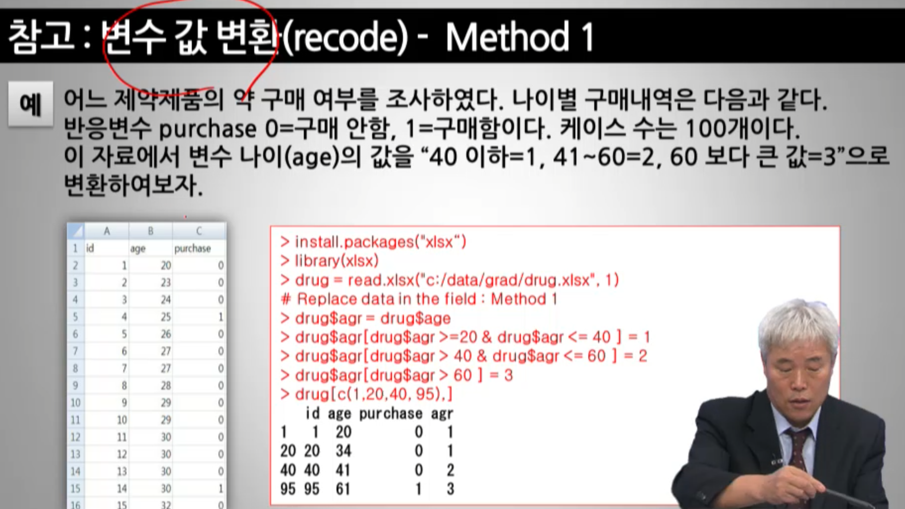
In [ ]:
- (범위별 매핑 -> )
recode=변수 값 변환이라고 한다.
- 새 변수를 만들고 (할당으로 복사)
- 인덱싱을 이용해서 범위별로 값 변환
변수갑 변환(recode) Method2 : car패키지의 recode()함수
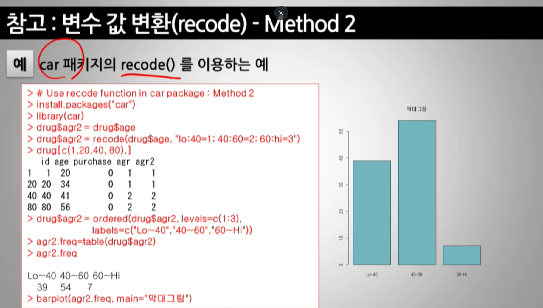
새 변수 만들어놓는 것은 똑같고
recode()함수를 이용하여범위를 간단하게 표현할 수 있다.- "
lo:40=1;40:60=2;60:hi=3"
- "
1,2,3 범주형 자료이면서 순서형 변수 순서를 ordered()를 이용해서 factor-라벨로 준다.
- 라벨을 주면 그래프에서도 나온다.
In [ ]:
값 라벨(Value labels): 숫자 -> 라벨로 바꾸기
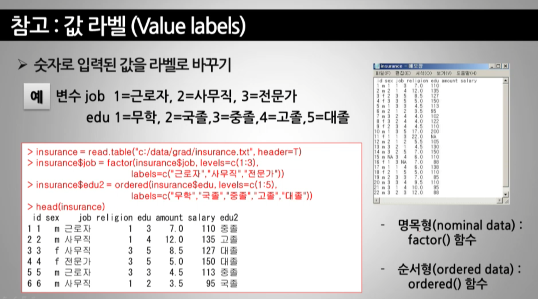
- 명목형 변수 -> 순서 없는 일반 범주
factor()를 이용해서 바꾼다. - 순서형 변수 -> 순서를 가진 범주
ordered()를 이용해서 바꾼다.
In [ ]: