Spatial operations and overlays: creating new geometries
In the previous notebook we have seen how to identify and use the spatial relationships between geometries. In this notebook, we will see how to create new geometries based on those relationships.
import pandas as pd
import geopandas
import matplotlib.pyplot as plt
countries = geopandas.read_file("data/ne_110m_admin_0_countries.zip")
cities = geopandas.read_file("data/ne_110m_populated_places.zip")
rivers = geopandas.read_file("data/ne_50m_rivers_lake_centerlines.zip")
# defining the same example geometries as in the previous notebook
belgium = countries.loc[countries['name'] == 'Belgium', 'geometry'].item()
brussels = cities.loc[cities['name'] == 'Brussels', 'geometry'].item()
Spatial operations
Next to the spatial predicates that return boolean values, Shapely and GeoPandas also provide operations that return new geometric objects.
Binary operations:
 |
 |
 |
 |
Buffer:
 |
 |
 |
 |
See https://shapely.readthedocs.io/en/stable/manual.html#spatial-analysis-methods for more details.
For example, using the toy data from above, let's construct a buffer around Brussels (which returns a Polygon):
geopandas.GeoSeries([belgium, brussels.buffer(1)]).plot(alpha=0.5, cmap='tab10')
and now take the intersection, union or difference of those two polygons:
brussels.buffer(1).intersection(belgium)
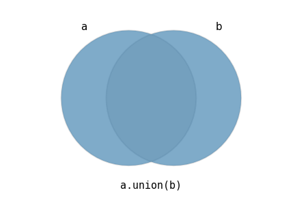
brussels.buffer(1).union(belgium)
brussels.buffer(1).difference(belgium)
Spatial operations with GeoPandas
Above we showed how to create a new geometry based on two individual shapely geometries. The same operations can be extended to GeoPandas. Given a GeoDataFrame, we can calculate the intersection, union or difference of each of the geometries with another geometry.
Let's look at an example with a subset of the countries. We have a GeoDataFrame with the country polygons of Africa, and now consider a rectangular polygon, representing an area around the equator:
africa = countries[countries.continent == 'Africa']
from shapely.geometry import LineString
box = LineString([(-10, 0), (50, 0)]).buffer(10, cap_style=3)
fig, ax = plt.subplots(figsize=(6, 6))
africa.plot(ax=ax, facecolor='none', edgecolor='k')
geopandas.GeoSeries([box]).plot(ax=ax, facecolor='C0', edgecolor='k', alpha=0.5)
The intersection method of the GeoDataFrame will now calculate the intersection with the rectangle for each of the geometries of the africa GeoDataFrame element-wise. Note that for many of the countries, those that do not overlap with the rectangle, this will be an empty geometry:
africa_intersection = africa.intersection(box)
africa_intersection.head()
What is returned is a new GeoSeries of the same length as the original dataframe, containing one row per country, but now containing only the intersection. In this example, the last element shown is an empty polygon, as that country was not overlapping with the box.
# remove the empty polygons before plotting
africa_intersection = africa_intersection[~africa_intersection.is_empty]
# plot the intersection
africa_intersection.plot()
Unary union and dissolve
Another useful method is the unary_union attribute, which converts the set of geometry objects in a GeoDataFrame into a single geometry object by taking the union of all those geometries.
For example, we can construct a single Shapely geometry object for the Africa continent:
africa_countries = countries[countries['continent'] == 'Africa']
africa = africa_countries.unary_union
africa
print(str(africa)[:1000])
Alternatively, you might want to take the unary union of a set of geometries but grouped by one of the attributes of the GeoDataFrame (so basically doing "groupby" + "unary_union"). For this operation, GeoPandas provides the dissolve() method:
continents = countries.dissolve(by="continent") # , aggfunc="sum"
continents
REMEMBER:
GeoPandas (and Shapely for the individual objects) provide a whole lot of basic methods to analyze the geospatial data (distance, length, centroid, boundary, convex_hull, simplify, transform, ....), much more than what we can touch in this tutorial.
An overview of all methods provided by GeoPandas can be found here: https://geopandas.readthedocs.io/en/latest/docs/reference.html
Let's practice!
EXERCISE 1: What are the districts close to the Seine?
Below, the coordinates for the Seine river in the neighborhood of Paris are provided as a GeoJSON-like feature dictionary (created at http://geojson.io).
Based on this seine object, we want to know which districts are located close (maximum 150 m) to the Seine.
- Create a buffer of 150 m around the Seine.
- Check which districts intersect with this buffered object.
- Make a visualization of the districts indicating which districts are located close to the Seine.
districts = geopandas.read_file("data/paris_districts.geojson").to_crs(epsg=2154)
# created a line with http://geojson.io
s_seine = geopandas.GeoDataFrame.from_features({"type":"FeatureCollection","features":[{"type":"Feature","properties":{},"geometry":{"type":"LineString","coordinates":[[2.408924102783203,48.805619828930226],[2.4092674255371094,48.81703747481909],[2.3927879333496094,48.82325391133874],[2.360687255859375,48.84912860497674],[2.338714599609375,48.85827758964043],[2.318115234375,48.8641501307046],[2.298717498779297,48.863246707697],[2.2913360595703125,48.859519915404825],[2.2594070434570312,48.8311646245967],[2.2436141967773438,48.82325391133874],[2.236919403076172,48.82347994904826],[2.227306365966797,48.828339513221444],[2.2224998474121094,48.83862215329593],[2.2254180908203125,48.84856379804802],[2.2240447998046875,48.85409863123821],[2.230224609375,48.867989496547864],[2.260265350341797,48.89192242750887],[2.300262451171875,48.910203080780285]]}}]},
                                               crs='EPSG:4326')
# convert to local UTM zone
s_seine_utm = s_seine.to_crs(epsg=2154)
import matplotlib.pyplot as plt
fig, ax = plt.subplots(figsize=(20, 10))
districts.plot(ax=ax, color='grey', alpha=0.4, edgecolor='k')
s_seine_utm.plot(ax=ax)
# access the single geometry object
seine = s_seine_utm.geometry.item()
seine
# %load _solved/solutions/04-spatial-operations-overlays1.py
# %load _solved/solutions/04-spatial-operations-overlays2.py
# %load _solved/solutions/04-spatial-operations-overlays3.py
EXERCISE 2: Exploring a Land Use dataset
For the following exercises, we first introduce a new dataset: a dataset about the land use of Paris (a simplified version based on the open European Urban Atlas). The land use indicates for what kind of activity a certain area is used, such as residential area or for recreation. It is a polygon dataset, with a label representing the land use class for different areas in Paris.
In this exercise, we will read the data, explore it visually, and calculate the total area of the different classes of land use in the area of Paris.
- Read in the
'paris_land_use.shp'file and assign the result to a variableland_use. - Make a plot of
land_use, using the'class'column to color the polygons. Add a legend withlegend=True, and make the figure size a bit larger. - Add a new column
'area'to the dataframe with the area of each polygon. - Calculate the total area in km² for each
'class'using thegroupby()method, and print the result.
Hints
- Reading a file can be done with the
geopandas.read_file()function. - To use a column to color the geometries, use the
columnkeyword to indicate the column name. - The area of each geometry can be accessed with the
areaattribute of thegeometryof the GeoDataFrame. - The
groupby()method takes the column name on which you want to group as the first argument.
# %load _solved/solutions/04-spatial-operations-overlays4.py
# %load _solved/solutions/04-spatial-operations-overlays5.py
# %load _solved/solutions/04-spatial-operations-overlays6.py
# %load _solved/solutions/04-spatial-operations-overlays7.py
EXERCISE 3: Intersection of two polygons
For this exercise, we are going to use 2 individual polygons: the district of Muette extracted from the districts dataset, and the green urban area of Boulogne, a large public park in the west of Paris, extracted from the land_use dataset. The two polygons have already been assigned to the muette and park_boulogne variables.
We first visualize the two polygons. You will see that they overlap, but the park is not fully located in the district of Muette. Let's determine the overlapping part:
- Plot the two polygons in a single map to examine visually the degree of overlap
- Calculate the intersection of the
park_boulogneandmuettepolygons. - Plot the intersection.
- Print the proportion of the area of the district that is occupied by the park.
Hints
- To plot single Shapely objects, you can put those in a
GeoSeries([..])to use the GeoPandasplot()method. - The intersection of to scalar polygons can be calculated with the
intersection()method of one of the polygons, and passing the other polygon as the argument to that method.
land_use = geopandas.read_file("data/paris_land_use.zip")
districts = geopandas.read_file("data/paris_districts.geojson").to_crs(land_use.crs)
# extract polygons
land_use['area'] = land_use.geometry.area
park_boulogne = land_use[land_use['class'] == "Green urban areas"].sort_values('area').geometry.iloc[-1]
muette = districts[districts.district_name == 'Muette'].geometry.item()
# Plot the two polygons
geopandas.GeoSeries([park_boulogne, muette]).plot(alpha=0.5, color=['green', 'blue'])
# %load _solved/solutions/04-spatial-operations-overlays8.py
# %load _solved/solutions/04-spatial-operations-overlays9.py
# %load _solved/solutions/04-spatial-operations-overlays10.py
EXERCISE 4: Intersecting a GeoDataFrame with a Polygon
Combining the land use dataset and the districts dataset, we can now investigate what the land use is in a certain district.
For that, we first need to determine the intersection of the land use dataset with a given district. Let's take again the Muette district as example case.
- Calculate the intersection of the
land_usepolygons with the singlemuettepolygon. Call the resultland_use_muette. - Remove the empty geometries from
land_use_muette. - Make a quick plot of this intersection, and pass
edgecolor='black'to more clearly see the boundaries of the different polygons. - Print the first five rows of
land_use_muette.
Hints
- The intersection of each geometry of a GeoSeries with another single geometry can be performed with the
intersection()method of a GeoSeries. - The
intersection()method takes as argument the geometry for which to calculate the intersection. - We can check which geometries are empty with the
is_emptyattribute of a GeoSeries.
land_use = geopandas.read_file("data/paris_land_use.zip")
districts = geopandas.read_file("data/paris_districts.geojson").to_crs(land_use.crs)
muette = districts[districts.district_name == 'Muette'].geometry.item()
# %load _solved/solutions/04-spatial-operations-overlays11.py
# %load _solved/solutions/04-spatial-operations-overlays12.py
# %load _solved/solutions/04-spatial-operations-overlays13.py
# %load _solved/solutions/04-spatial-operations-overlays14.py
# %load _solved/solutions/04-spatial-operations-overlays15.py
You can see in the plot that we now only have a subset of the full land use dataset. The original land_use_muette (before removing the empty geometries) still has the same number of rows as the original land_use, though. But many of the rows, as you could see by printing the first rows, consist now of empty polygons when it did not intersect with the Muette district.
The intersection() method also returned only geometries. If we want to combine those intersections with the attributes of the original land use, we can take a copy of this and replace the geometries with the intersections (you can uncomment and run to see the code):
# %load _solved/solutions/04-spatial-operations-overlays16.py
# %load _solved/solutions/04-spatial-operations-overlays17.py
# %load _solved/solutions/04-spatial-operations-overlays18.py
EXERCISE 5: The land use of the Muette district
Based on the land_use_muette dataframe with the land use for the Muette districts as calculated above, we can now determine the total area of the different land use classes in the Muette district.
- Calculate the total area per land use class.
- Calculate the fraction (in percentage) for the different land use classes.
Hints
- The intersection of each geometry of a GeoSeries with another single geometry can be performed with the
intersection()method of a GeoSeries. - The
intersection()method takes as argument the geometry for which to calculate the intersection. - We can check which geometries are empty with the
is_emptyattribute of a GeoSeries.
# %load _solved/solutions/04-spatial-operations-overlays19.py
# %load _solved/solutions/04-spatial-operations-overlays20.py
The above was only for a single district. If we want to do this more easily for all districts, we can do this with the overlay operation.
The overlay operation
In a spatial join operation, we are not changing the geometries itself. We are not joining geometries, but joining attributes based on a spatial relationship between the geometries. This also means that the geometries need to at least overlap partially.
If you want to create new geometries based on joining (combining) geometries of different dataframes into one new dataframe (eg by taking the intersection of the geometries), you want an overlay operation.
How does it differ compared to the intersection method?
With the intersection() method introduced in the previous section, we could for example determine the intersection of a set of countries with another polygon, a circle in the example below:

However, this method (countries.intersection(circle)) also has some limitations.
- Mostly useful when intersecting a GeoSeries with a single polygon.
- Does not preserve attribute information of the intersecting polygons.
For cases where we require a bit more complexity, it is preferable to use the "overlay" operation, instead of the intersection method.
Consider the following simplified example. On the left we see again the 3 countries. On the right we have the plot of a GeoDataFrame with some simplified geologic regions for the same area:
 |
 |
By simply plotting them on top of each other, as shown below, you can see that the polygons of both layers intersect.
But now, by "overlaying" the two layers, we can create a third layer that contains the result of intersecting both layers: all the intersections of each country with each geologic region. It keeps only those areas that were included in both layers.
 |
 |
This operation is called an intersection overlay, and in GeoPandas we can perform this operation with the geopandas.overlay() function.
Another code example:
africa = countries[countries['continent'] == 'Africa']
africa.plot()
cities['geometry'] = cities.buffer(2)
intersection = geopandas.overlay(africa, cities, how='intersection')
intersection.plot()
intersection.head()
With the overlay method, we pass the full GeoDataFrame with all regions to intersect the countries with. The result contains all non-empty intersections of all combinations of countries and city regions.
Note that the result of the overlay function also keeps the attribute information of both the countries as the city regions. That can be very useful for further analysis.
geopandas.overlay(africa, cities, how='intersection').plot() # how="difference"/"union"/"symmetric_difference"
- Spatial join: transfer attributes from one dataframe to another based on the spatial relationship
- Spatial overlay: construct new geometries based on spatial operation between both dataframes (and combining attributes of both dataframes)
Let's practice!
EXERCISE 6: Overlaying spatial datasets I
We will now combine both datasets in an overlay operation. Create a new GeoDataFrame consisting of the intersection of the land use polygons which each of the districts, but make sure to bring the attribute data from both source layers.
- Create a new GeoDataFrame from the intersections of
land_useanddistricts. Assign the result to a variablecombined. - Print the first rows the resulting GeoDataFrame (
combined).
Hints
- The intersection of two GeoDataFrames can be calculated with the
geopandas.overlay()function. - The
overlay()functions takes first the two GeoDataFrames to combine, and a thirdhowkeyword indicating how to combine the two layers. - For making an overlay based on the intersection, you can pass
how='intersection'.
land_use = geopandas.read_file("data/paris_land_use.zip")
districts = geopandas.read_file("data/paris_districts.geojson").to_crs(land_use.crs)
# %load _solved/solutions/04-spatial-operations-overlays21.py
# %load _solved/solutions/04-spatial-operations-overlays22.py
EXERCISE 7: Overlaying spatial datasets II
Now that we created the overlay of the land use and districts datasets, we can more easily inspect the land use for the different districts. Let's get back to the example district of Muette, and inspect the land use of that district.
- Add a new column
'area'with the area of each polygon to thecombinedGeoDataFrame. - Create a subset called
land_use_muettewhere the'district_name'is equal to "Muette". - Make a plot of
land_use_muette, using the'class'column to color the polygons. - Calculate the total area for each
'class'ofland_use_muetteusing thegroupby()method, and print the result.
Hints
- The area of each geometry can be accessed with the
areaattribute of thegeometryof the GeoDataFrame. - To use a column to color the geometries, pass its name to the
columnkeyword. - The
groupby()method takes the column name on which you want to group as the first argument. - The total area for each class can be calculated by taking the
sum()of the area.
# %load _solved/solutions/04-spatial-operations-overlays23.py
# %load _solved/solutions/04-spatial-operations-overlays24.py
# %load _solved/solutions/04-spatial-operations-overlays25.py
# %load _solved/solutions/04-spatial-operations-overlays26.py
EXERCISE 8: Overlaying spatial datasets III
Thanks to the result of the overlay operation, we can now more easily perform a similar analysis for all districts. Let's investigate the fraction of green urban area in each of the districts.
- Based on the
combineddataset, calculate the total area per district usinggroupby(). - Select the subset of "Green urban areas" from
combinedand call thisurban_green. - Now calculate the total area per district for this
urban_greensubset, and call thisurban_green_area. - Determine the fraction of urban green area in each district.
# %load _solved/solutions/04-spatial-operations-overlays27.py
# %load _solved/solutions/04-spatial-operations-overlays28.py
# %load _solved/solutions/04-spatial-operations-overlays29.py
# %load _solved/solutions/04-spatial-operations-overlays30.py
# %load _solved/solutions/04-spatial-operations-overlays31.py
# %load _solved/solutions/04-spatial-operations-overlays32.py
An alternative to calculate the area per land use class in each district:
combined.groupby(["district_name", "class"])["area"].sum().reset_index()