Information Engines¶

Neil D. Lawrence¶

2025-04-15¶

Abstract: The relationship between physical systems and intelligence has long fascinated researchers in computer science and physics. This talk explores fundamental connections between thermodynamic systems and intelligent decision-making through the lens of free energy principles.

We examine how concepts from statistical mechanics - particularly the relationship between total energy, free energy, and entropy - might provide novel insights into the nature of intelligence and learning. By drawing parallels between physical systems and information processing, we consider how measurement and observation can be viewed as processes that modify available energy. The discussion encompasses how model approximations and uncertainties might be understood through thermodynamic analogies, and explores the implications of treating intelligence as an energy-efficient state-change process.

While these connections remain speculative, they offer intriguing perspectives for discussing the fundamental nature of intelligence and learning systems. The talk aims to stimulate discussion about these potential relationships rather than present definitive conclusions.

::: {.cell .markdown}

Hydrodynamica¶

[edit]

When Laplace spoke of the curve of a simple molecule of air, he may well have been thinking of Daniel Bernoulli (1700-1782). Daniel Bernoulli was one name in a prodigious family. His father and brother were both mathematicians. Daniel’s main work was known as Hydrodynamica.

Figure: Daniel Bernoulli’s Hydrodynamica published in 1738. It was one of the first works to use the idea of conservation of energy. It used Newton’s laws to predict the behaviour of gases.

Daniel Bernoulli described a kinetic theory of gases, but it wasn’t until 170 years later when these ideas were verified after Einstein had proposed a model of Brownian motion which was experimentally verified by Jean Baptiste Perrin.

Figure: Daniel Bernoulli’s chapter on the kinetic theory of gases, for a review on the context of this chapter see Mikhailov (n.d.). For 1738 this is extraordinary thinking. The notion of kinetic theory of gases wouldn’t become fully accepted in Physics until 1908 when a model of Einstein’s was verified by Jean Baptiste Perrin.

Entropy Billiards¶

[edit]

Entropy:

0.0000

New Ball

Pause

Skip 1000s

Histogram

Figure: Bernoulli’s simple kinetic models of gases assume that the molecules of air operate like billiard balls.

Another important figure for Cambridge was the first to derive the probability distribution that results from small balls banging together in this manner. In doing so, James Clerk Maxwell founded the field of statistical physics.

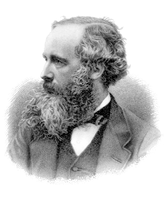
Figure: James Clerk Maxwell 1831-1879 Derived distribution of velocities of particles in an ideal gas (elastic fluid).

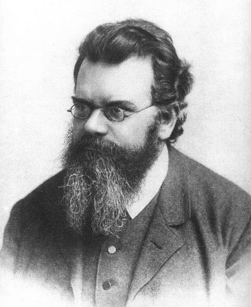
Figure: James Clerk Maxwell (1831-1879), Ludwig Boltzmann (1844-1906) Josiah Willard Gibbs (1839-1903)

Many of the ideas of early statistical physicists were rejected by a cadre of physicists who didn’t believe in the notion of a molecule. The stress of trying to have his ideas established caused Boltzmann to commit suicide in 1906, only two years before the same ideas became widely accepted.

Figure: Boltzmann’s paper Boltzmann (n.d.) which introduced the relationship between entropy and probability. A translation with notes is available in Sharp and Matschinsky (2015).

The important point about the uncertainty being represented here is that it is not genuine stochasticity, it is a lack of knowledge about the system. The techniques proposed by Maxwell, Boltzmann and Gibbs allow us to exactly represent the state of the system through a set of parameters that represent the sufficient statistics of the physical system. We know these values as the volume, temperature, and pressure. The challenge for us, when approximating the physical world with the techniques we will use is that we will have to sit somewhere between the deterministic and purely stochastic worlds that these different scientists described.

One ongoing characteristic of people who study probability and uncertainty is the confidence with which they hold opinions about it. Another leader of the Cavendish laboratory expressed his support of the second law of thermodynamics (which can be proven through the work of Gibbs/Boltzmann) with an emphatic statement at the beginning of his book.

Figure: Eddington’s book on the Nature of the Physical World (Eddington, 1929)

The same Eddington is also famous for dismissing the ideas of a young Chandrasekhar who had come to Cambridge to study in the Cavendish lab. Chandrasekhar demonstrated the limit at which a star would collapse under its own weight to a singularity, but when he presented the work to Eddington, he was dismissive suggesting that there “must be some natural law that prevents this abomination from happening”.

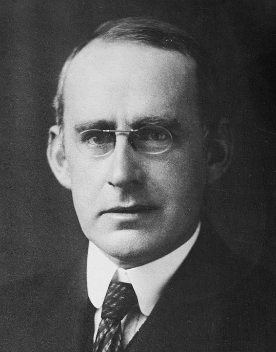
Figure: Chandrasekhar (1910-1995) derived the limit at which a star collapses in on itself. Eddington’s confidence in the 2nd law may have been what drove him to dismiss Chandrasekhar’s ideas, humiliating a young scientist who would later receive a Nobel prize for the work.

Figure: Eddington makes his feelings about the primacy of the second law clear. This primacy is perhaps because the second law can be demonstrated mathematically, building on the work of Maxwell, Gibbs and Boltzmann. Eddington (1929)

Presumably he meant that the creation of a black hole seemed to transgress the second law of thermodynamics, although later Hawking was able to show that blackholes do evaporate, but the time scales at which this evaporation occurs is many orders of magnitude slower than other processes in the universe.

Maxwell’s Demon¶

[edit]

Maxwell’s demon is a thought experiment described by James Clerk Maxwell in his book, Theory of Heat (Maxwell, 1871) on page 308.

But if we conceive a being whose faculties are so sharpened that he can follow every molecule in its course, such a being, whose attributes are still as essentially finite as our own, would be able to do what is at present impossible to us. For we have seen that the molecules in a vessel full of air at uniform temperature are moving with velocities by no means uniform, though the mean velocity of any great number of them, arbitrarily selected, is almost exactly uniform. Now let us suppose that such a vessel is divided into two portions, A and B, by a division in which there is a small hole, and that a being, who can see the individual molecules, opens and closes this hole, so as to allow only the swifter molecules to pass from A to B, and the only the slower ones to pass from B to A. He will thus, without expenditure of work, raise the temperature of B and lower that of A, in contradiction to the second law of thermodynamics.

James Clerk Maxwell in Theory of Heat (Maxwell, 1871) page 308

He goes onto say:

This is only one of the instances in which conclusions which we have draw from our experience of bodies consisting of an immense number of molecules may be found not to be applicable to the more delicate observations and experiments which we may suppose made by one who can perceive and handle the individual molecules which we deal with only in large masses

Figure: Maxwell’s demon was designed to highlight the statistical nature of the second law of thermodynamics.

Entropy:

0.0000

New Ball

Pause

Skip 1000s

Histogram

Figure: Maxwell’s Demon. The demon decides balls are either cold (blue) or hot (red) according to their velocity. Balls are allowed to pass the green membrane from right to left only if they are cold, and from left to right, only if they are hot.

Maxwell’s demon allows us to connect thermodynamics with information theory (see e.g. Hosoya et al. (2015);Hosoya et al. (2011);Bub (2001);Brillouin (1951);Szilard (1929)). The connection arises due to a fundamental connection between information erasure and energy consumption Landauer (1961).

Alemi and Fischer (2019)

Information Theory and Thermodynamics¶

[edit]

Information theory provides a mathematical framework for quantifying information. Many of information theory’s core concepts parallel those found in thermodynamics. The theory was developed by Claude Shannon who spoke extensively to MIT’s Norbert Wiener at while it was in development (Conway and Siegelman, 2005). Wiener’s own ideas about information were inspired by Willard Gibbs, one of the pioneers of the mathematical understanding of free energy and entropy. Deep connections between physical systems and information processing have connected information and energy from the start.

Entropy¶

Shannon’s entropy measures the uncertainty or unpredictability of information content. This mathematical formulation is inspired by thermodynamic entropy, which describes the dispersal of energy in physical systems. Both concepts quantify the number of possible states and their probabilities.

Figure: Maxwell’s demon thought experiment illustrates the relationship between information and thermodynamics.

In thermodynamics, free energy represents the energy available to do work. A system naturally evolves to minimize its free energy, finding equilibrium between total energy and entropy. Free energy principles are also pervasive in variational methods in machine learning. They emerge from Bayesian approaches to learning and have been heavily promoted by e.g. Karl Friston as a model for the brain.

The relationship between entropy and Free Energy can be explored through the Legendre transform. This is most easily reviewed if we restrict ourselves to distributions in the exponential family.

Exponential Family¶

The exponential family has the form

$$\rho(Z) = h(Z) \exp\left(\boldsymbol{\theta}^\top T(Z) + A(\boldsymbol{\theta})\right)$$ where $h(Z)$ is the base measure, $\boldsymbol{\theta}$ is the natural parameters, $T(Z)$ is the sufficient statistics and $A(\boldsymbol{\theta})$ is the log partition function. Its entropy can be computed as $$S(Z) = A(\boldsymbol{\theta}) - \boldsymbol{\theta}^\top \nabla_\boldsymbol{\theta}A(\boldsymbol{\theta}) - E_{\rho(Z)}\left[\log h(Z)\right],$$ where $E_{\rho(Z)}[\cdot]$ is the expectation under the distribution $\rho(Z)$.

Available Energy¶

Work through Measurement¶

In machine learning and Bayesian inference, the Markov blanket is the set of variables that are conditionally independent of the variable of interest given the other variables. To introduce this idea into our information system, we first split the system into two parts, the variables, $X$, and the memory $M$.

The variables are the portion of the system that is stochastically evolving over time. The memory is a low entropy partition of the system that will give us knowledge about this evolution.

We can now write the joint entropy of the system in terms of the mutual information between the variables and the memory.

$$S(Z) = S(X,M) = S(X|M) + S(M) = S(X) - I(X;M) + S(M).$$ This gives us the first hint at the connection between information and energy.

If $M$ is viewed as a measurement then the change in entropy of the system before and after measurement is given by $S(X|M) - S(X)$ wehich is given by $-I(X;M)$. This is implies that measurement increases the amount of available energy we obtain from the system (Parrondo et al., 2015).

The difference in available energy is given by

$$\Delta A = A(X) - A(Z|M) = I(X;M),$$ where we note that the resulting system is no longer in thermodynamic equilibrium due to the low entropy of the memory.

The Animal Game¶

[edit]

The Entropy Game is a framework for understanding efficient uncertainty reduction. To start think of finding the optimal strategy for identifying an unknown entity by asking the minimum number of yes/no questions.

The 20 Questions Paradigm¶

In the game of 20 Questions player one (Alice) thinks of an object, player two (Bob) must identify it by asking at most 20 yes/no questions. The optimal strategy is to divide the possibility space in half with each question. The binary search approach ensures maximum information gain with each inquiry and can access $2^20$ or about a million different objects.

Figure: The optimal strategy in the Entropy Game resembles a binary search, dividing the search space in half with each question.

Entropy Reduction and Decisions¶

From an information-theoretic perspective, decisions can be taken in a way that efficiently reduces entropy - our the uncertainty about the state of the world. Each observation or action an intelligent agent takes should maximize expected information gain, optimally reducing uncertainty given available resources.

The entropy before the question is $S(X)$. The entropy after the question is $S(X|M)$. The information gain is the difference between the two, $I(X;M) = S(X) - S(X|M)$. Optimal decision making systems maximize this information gain per unit cost.

Thermodynamic Parallels¶

The entropy game connects decision-making to thermodynamics.

This perspective suggests a profound connection: intelligence might be understood as a special case of systems that efficiently extract, process, and utilize free energy from their environments, with thermodynamic principles setting fundamental constraints on what’s possible.

Information Engines: Intelligence as an Energy-Efficiency¶

[edit]

The entropy game shows some parallels between thermodynamics and measurement. This allows us to imagine information engines, simple systems that convert information to energy. This is our first simple model of intelligence.

Measurement as a Thermodynamic Process: Information-Modified Second Law¶

The second law of thermodynamics was generalised to include the effect of measurement by Sagawa and Ueda (Sagawa and Ueda, 2008). They showed that the maximum extractable work from a system can be increased by $k_BTI(X;M)$ where $k_B$ is Boltzmann’s constant, $T$ is temperature and $I(X;M)$ is the information gained by making a measurement, $M$,

$$I(X;M) = \sum_{x,m} \rho(x,m) \log \frac{\rho(x,m)}{\rho(x)\rho(m)},$$ where $\rho(x,m)$ is the joint probability of the system and measurement (see e.g. eq 14 in Sagawa and Ueda (2008)). This can be written as $$W_\text{ext} \leq - \Delta\mathcal{F} + k_BTI(X;M),$$ where $W_\text{ext}$ is the extractable work and it is upper bounded by the negative change in free energy, $\Delta \mathcal{F}$, plus the energy gained from measurement, $k_BTI(X;M)$. This is the information-modified second law.

The measurements can be seen as a thermodynamic process. In theory measurement, like computation is reversible. But in practice the process of measurement is likely to erode the free energy somewhat, but as long as the energy gained from information, $kTI(X;M)$ is greater than that spent in measurement the pricess can be thermodynamically efficient.

The modified second law shows that the maximum additional extractable work is proportional to the information gained. So information acquisition creates extractable work potential. Thermodynamic consistency is maintained by properly accounting for information-entropy relationships.

Efficacy of Feedback Control¶

Sagawa and Ueda extended this relationship to provide a generalised Jarzynski equality for feedback processes (Sagawa and Ueda, 2010). The Jarzynski equality is an imporant result from nonequilibrium thermodynamics that relates the average work done across an ensemble to the free energy difference between initial and final states (Jarzynski, 1997),

$$\left\langle \exp\left(-\frac{W}{k_B T}\right) \right\rangle = \exp\left(-\frac{\Delta\mathcal{F}}{k_BT}\right),$$ where $\langle W \rangle$ is the average work done across an ensemble of trajectories, $\Delta\mathcal{F}$ is the change in free energy, $k_B$ is Boltzmann’s constant, and $\Delta S$ is the change in entropy. Sagawa and Ueda extended this equality to to include information gain from measurement (Sagawa and Ueda, 2010), $$\left\langle \exp\left(-\frac{W}{k_B T}\right) \exp\left(\frac{\Delta\mathcal{F}}{k_BT}\right) \exp\left(-\mathcal{I}(X;M)\right)\right\rangle = 1,$$ where $\mathcal{I}(X;M) = \log \frac{\rho(X|M)}{\rho(X)}$ is the information gain from measurement, and the mutual information is recovered $I(X;M) = \left\langle \mathcal{I}(X;M) \right\rangle$ as the average information gain.

Sagawa and Ueda introduce an efficacy term that captures the effect of feedback on the system they note in the presence of feedback,

$$\left\langle \exp\left(-\frac{W}{k_B T}\right) \exp\left(\frac{\Delta\mathcal{F}}{k_BT}\right)\right\rangle = \gamma,$$ where $\gamma$ is the efficacy.

Channel Coding Perspective on Memory¶

When viewing $M$ as an information channel between past and future states, Shannon’s channel coding theorems apply (Shannon, 1948). The channel capacity $C$ represents the maximum rate of reliable information transmission [ C = _{(M)} I(X_1;M) ] and for a memory of $n$ bits we have [ C n, ] as the mutual information is upper bounded by the entropy of $\rho(M)$ which is at most $n$ bits.

This relationship seems to align with Ashby’s Law of Requisite Variety (pg 229 Ashby (1952)), which states that a control system must have at least as much ‘variety’ as the system it aims to control. In the context of memory systems, this means that to maintain temporal correlations effectively, the memory’s state space must be at least as large as the information content it needs to preserve. This provides a lower bound on the necessary memory capacity that complements the bound we get from Shannon for channel capacity.

This helps determine the required memory size for maintaining temporal correlations, optimal coding strategies, and fundamental limits on temporal correlation preservation.

Decomposition into Past and Future¶

Model Approximations and Thermodynamic Efficiency¶

Intelligent systems must balance measurement against energy efficiency and time requirements. A perfect model of the world would require infinite computational resources and speed, so approximations are necessary. This leads to uncertainties. Thermodynamics might be thought of as the physics of uncertainty: at equilibrium thermodynamic systems find thermodynamic states that minimize free energy, equivalent to maximising entropy.

Markov Blanket¶

To introduce some structure to the model assumption. We split $X$ into $X_0$ and $X_1$. $X_0$ is past and present of the system, $X_1$ is future The conditional mutual information $I(X_0;X_1|M)$ which is zero if $X_1$ and $X_0$ are independent conditioned on $M$.

At What Scales Does this Apply?¶

The equipartition theorem tells us that at equilibrium the average energy is $kT/2$ per degree of freedom. This means that for systems that operate at “human scale” the energy involved is many orders of magnitude larger than the amount of information we can store in memory. For a car engine producing 70 kW of power at 370 Kelvin, this implies

$$\frac{2 \times 70,000}{370 \times k_B} = \frac{2 \times 70,000}{370\times 1.380649×10^{−23}} = 2.74 × 10^{25}$$ degrees of freedom per second. If we make a conservative assumption of one bit per degree of freedom, then the mutual information we would require in one second for comparative energy production would be around 3400 zettabytes, implying a memory bandwidth of around 3,400 zettabytes per second. In 2025 the estimate of all the data in the world stands at 149 zettabytes.

Small-Scale Biochemical Systems and Information Processing¶

While macroscopic systems operate in regimes where traditional thermodynamics dominates, microscopic biological systems operate at scales where information and thermal fluctuations become critically important. Here we examine how the framework applies to molecular machines and processes that have evolved to operate efficiently at these scales.

Molecular machines like ATP synthase, kinesin motors, and the photosynthetic apparatus can be viewed as sophisticated information engines that convert energy while processing information about their environment. These systems have evolved to exploit thermal fluctuations rather than fight against them, using information processing to extract useful work.

ATP Synthase: Nature’s Rotary Engine¶

ATP synthase functions as a rotary molecular motor that synthesizes ATP from ADP and inorganic phosphate using a proton gradient. The system uses the proton gradient as both an energy source and an information source about the cell’s energetic state and exploits Brownian motion through a ratchet mechanism. It converts information about proton locations into mechanical rotation and ultimately chemical energy with approximately 3-4 protons required per ATP.

Estimates suggest that one synapse firing may require $10^4$ ATP molecules, so around $4 \times 10^4$ protons. If we take the human brain as containing around $10^{14}$ synapses, and if we suggest each synapse only fires about once every five seconds, we would require approximately $10^{18}$ protons per second to power the synapses in our brain. With each proton having six degrees of freedom. Under these rough calculations the memory capacity distributed across the ATP Synthase in our brain must be of order $6 \times 10^{18}$ bits per second or 750 petabytes of information per second. Of course this memory capacity would be devolved across the billions of neurons within hundreds or thousands of mitochondria that each can contain thousands of ATP synthase molecules. By composition of extremely small systems we can see it’s possible to improve efficiencies in ways that seem very impractical for a car engine.

Quick note to clarify, here we’re referring to the information requirements to make our brain more energy efficient in its information processing rather than the information processing capabilities of the neurons themselves!

Jaynes’s Maximum Entropy Principle¶

[edit]

In his seminal 1957 paper (Jaynes, 1957), Ed Jaynes proposed a foundation for statistical mechanics based on information theory. Rather than relying on ergodic hypotheses or ensemble interpretations, Jaynes recast that the problem of assigning probabilities in statistical as a problem of inference with incomplete information.

A central problem in statistical mechanics is assigning initial probabilities when our knowledge is incomplete. For example, if we know only the average energy of a system, what probability distribution should we use? Jaynes argued that we should use the distribution that maximizes entropy subject to the constraints of our knowledge.

Jaynes illustrated the approachwith a simple example: Suppose a die has been tossed many times, with an average result of 4.5 rather than the expected 3.5 for a fair die. What probability assignment $P_n$ ($n=1,2,...,6$) should we make for the next toss?

We need to satisfy two constraints

Many distributions could satisfy these constraints, but which one makes the fewest unwarranted assumptions? Jaynes argued that we should choose the distribution that is maximally noncommittal with respect to missing information - the one that maximizes the entropy, This principle leads to the exponential family of distributions, which in statistical mechanics gives us the canonical ensemble and other familiar distributions.

The General Maximum-Entropy Formalism¶

For a more general case, suppose a quantity $x$ can take values $(x_1, x_2, \ldots, x_n)$ and we know the average values of several functions $f_k(x)$. The problem is to find the probability assignment $p_i = p(x_i)$ that satisfies and maximizes the entropy $S_I = -\sum_{i=1}^n p_i \log p_i$.

Using Lagrange multipliers, the solution is the generalized canonical distribution, where $Z(\lambda_1,\ldots,\lambda_m)$ is the partition function, The Lagrange multipliers $\lambda_k$ are determined by the constraints, The maximum attainable entropy is

Jaynes’ World¶

[edit]

Jaynes’ World is a zero-player game that implements a version of the entropy game. The dynamical system is defined by a distribution, $\rho(Z)$, over a state space $Z$. The state space is partitioned into observable variables $X$ and memory variables $M$. The memory variables are considered to be in an information resevoir, a thermodynamic system that maintains information in an ordered state (see e.g. Barato and Seifert (2014)). The entropy of the whole system is bounded below by 0 and above by $N$. So the entropy forms a compact manifold with respect to its parameters.

Unlike the animal game, where decisions are made by reducing entropy at each step, our system evovles mathematically by maximising the instantaneous entropy production. Conceptually we can think of this as ascending the gradient of the entropy, $S(Z)$.

In the animal game the questioner starts with maximum uncertainty and targets minimal uncertainty. Jaynes’ world starts with minimal uncertainty and aims for maximum uncertainty.

We can phrase this as a thought experiment. Imagine you are in the game, at a given turn. You want to see where the game came from, so you look back across turns. The direction the game came from is now the direction of steepest descent. Regardless of where the game actually started it looks like it started at a minimal entropy configuration that we call the origin. Similarly, wherever the game is actually stopped there will nevertheless appear to be an end point we call end that will be a configuration of maximal entropy, $N$.

This speculation allows us to impose the functional form of our proability distribution. As Jaynes has shown (Jaynes, 1957), the stationary points of a free-form optimisation (minimum or maximum) will place the distribution in the, $\rho(Z)$ in the exponential family,

$$\rho(Z) = h(Z) \exp(\boldsymbol{\theta}^\top T(Z) - A(\boldsymbol{\theta})),$$ where $h(Z)$ is the base measure, $T(Z)$ are sufficient statistics, $A(\boldsymbol{\theta})$ is the log-partition function, $\boldsymbol{\theta}$ are the natural parameters of the distribution.}

This constraint to the exponential family is highly convenient as we will rely on it heavily for the dynamics of the game. In particular, by focussing on the natural parameters we find that we are optimising within an information geometry (Amari, 2016). In exponential family distributions, the entropy gradient is given by,

$$\nabla_{\boldsymbol{\theta}}S(Z) = \mathbf{g} = \nabla^2_\boldsymbol{\theta} A(\boldsymbol{\theta}(M))$$ And the Fisher information matrix, $G(\boldsymbol{\theta})$, is also the Hessian of the manifold, $$G(\boldsymbol{\theta}) = \nabla^2_{\boldsymbol{\theta}} A(\boldsymbol{\theta}) = \text{Cov}[T(Z)].$$ Traditionally, when optimising on an information geometry we take natural gradient steps, equivalen to a Newton minimisation step, $$\Delta \boldsymbol{\theta} = - G(\boldsymbol{\theta})^{-1} \mathbf{g},$$ but this is not the direction that gives the instantaneious maximisation of the entropy production, instead our gradient step is given by $$\Delta \boldsymbol{\theta} = \eta \mathbf{g},$$ where $\eta$ is a ‘learning rate’.

System Evolution¶

We are now in a position to summarise the start state and the end state of our system, as well as to speculate on the nature of the transition between the two states.

Start State¶

The origin configuration is a low entropy state, with value near the lower bound of 0. The information is highly structured, by definition we place all variables in $M$, the information resevoir at this time. The uncertainty principle is present to handle the competeing needs of precision in parameters (giving us the near-singular form for $\boldsymbol{\theta}(M)$, and capacity in the information channel that $M$ provides (the capacity $c(\boldsymbol{\theta})$ is upper bounded by $S(M)$.

End State¶

The end configuration is a high entropy state, near the upper bound. Both the minimal entropy and maximal entropy states are revealed by Ed Jaynes’ variational minimisation approach and are in the exponential family. In many cases a version of Zeno’s paradox will arise where the system asymtotes to the final state, taking smaller steps at each time. At this point the system is at equilibrium.

From Maximum to Minimal Entropy¶

[edit]

Jaynes formulated his principle in terms of maximizing entropy, we can also view certain problems as minimizing entropy under appropriate constraints. The duality becomes apparent when we consider the relationship between entropy and information.

The maximum entropy principle finds the distribution that is maximally noncommittal given certain constraints. Conversely, we can seek the distribution that minimizes entropy subject to different constraints - this represents the distribution with maximum structure or information.

Consider the uncertainty principle. When we seek states that minimize the product of position and momentum uncertainties, we are seeking minimal entropy states subject to the constraint of the uncertainty principle.

The mathematical formalism remains the same, but with different constraints and optimization direction, where $g_k$ are functions representing constraints different from simple averages.

The solution still takes the form of an exponential family, where $\mu_k$ are Lagrange multipliers for the constraints.

Minimal Entropy States in Quantum Systems¶

The pure states of quantum mechanics are those that minimize von Neumann entropy $S = -\text{Tr}(\rho \log \rho)$ subject to the constraints of quantum mechanics.

For example, coherent states minimize the entropy subject to constraints on the expectation values of position and momentum operators. These states achieve the minimum uncertainty allowed by quantum mechanics.

Histogram Game¶

[edit]

To illustrate the concept of the Jaynes’ world entropy game we’ll run a simple example using a four bin histogram. The entropy of a four bin histogram can be computed as,

$$S(p) = - \sum_{i=1}^4 p_i \log_2 p_i.$$

First we write some helper code to plot the histogram and compute its entropy.

We can compute the entropy of any given histogram.

Figure: The entropy of a four bin histogram.

We can play the entropy game by starting with a histogram with all the probability mass in the first bin and then ascending the gradient of the entropy function.

Two-Bin Histogram Example¶

[edit]

The simplest possible example of Jaynes’ World is a two-bin histogram with probabilities $p$ and $1-p$. This minimal system allows us to visualize the entire entropy landscape.

The natural parameter is the log odds, $\theta = \log\frac{p}{1-p}$, and the update given by the entropy gradient is

$$\Delta \theta_{\text{steepest}} = \eta \frac{\text{d}S}{\text{d}\theta} = \eta p(1-p)(\log(1-p) - \log p).$$ The Fisher information is $$G(\theta) = p(1-p)$$ This creates a dynamic where as $p$ approaches either 0 or 1 (minimal entropy states), the Fisher information approaches zero, creating a critical slowing” effect. This critical slowing is what leads to the formation of information resevoirs. Note also that in the natural gradient the updated is given by multiplying the gradient by the inverse Fisher information, which would lead to a more efficient update of the form, $$\Delta \theta_{\text{natural}} = \eta(\log(1-p) - \log p),$$ however, it is this efficiency that we want our game to avoid, because it is the inefficient behaviour in the reagion of saddle points that leads to critical slowing and the emergence of information resevoirs.

Figure: Entropy gradients of the two bin histogram agains position.

This example reveals the entropy extrema at $p = 0$, $p = 0.5$, and $p = 1$. At minimal entropy ($p \approx 0$ or $p \approx 1$), the gradient approaches zero, creating natural information reservoirs. The dynamics slow dramatically near these points - these are the areas of critical slowing that create information reservoirs.

Gradient Ascent in Natural Parameter Space¶

We can visualize the entropy maximization process by performing gradient ascent in the natural parameter space $\theta$. Starting from a low-entropy state, we follow the gradient of entropy with respect to $\theta$ to reach the maximum entropy state.

Figure: Evolution of the two-bin histogram during gradient ascent in natural parameter space.

Figure: Entropy evolution during gradient ascent for the two-bin histogram.

Figure: Gradient ascent trajectory in the natural parameter space for the two-bin histogram.

The gradient ascent visualization shows how the system evolves in the natural parameter space $\theta$. Starting from a negative $\theta$ (corresponding to a low-entropy state with $p << 0.5$), the system follows the gradient of entropy with respect to $\theta$ until it reaches $\theta = 0$ (corresponding to $p = 0.5$), which is the maximum entropy state.

Note that the maximum entropy occurs at $\theta = 0$, which corresponds to $p = 0.5$. The gradient of entropy with respect to $\theta$ is zero at this point, making it a stable equilibrium for the gradient ascent process.

Uncertainty Principle¶

[edit]

One challenge is how to parameterise our exponential family. We’ve mentioned that the variables $Z$ are partitioned into observable variables $X$ and memory variables $M$. Given the minimal entropy initial state, the obvious initial choice is that at the origin all variables, $Z$, should be in the information reservoir, $M$. This implies that they are well determined and present a sensible choice for the source of our parameters.

We define a mapping, $\boldsymbol{\theta}(M)$, that maps the information resevoir to a set of values that are equivalent to the natural parameters. If the entropy of these parameters is low, and the distribution $\rho(\boldsymbol{\theta})$ is sharply peaked then we can move from treating the memory mapping, $\boldsymbol{\theta}(\cdot)$, as a random processe to an assumption that it is a deterministic function. We can then follow gradients with respect to these $\boldsymbol{\theta}$ values.

This allows us to rewrite the distribution over $Z$ in a conditional form,

$$\rho(X|M) = h(X) \exp(\boldsymbol{\theta}(M)^\top T(X) - A(\boldsymbol{\theta}(M))).$$

Unfortunately this assumption implies that $\boldsymbol{\theta}(\cdot)$ is a delta function, and since our representation as a compact manifold (bounded below by $0$ and above by $N$) it does not admit any such singularities.

Capacity $\leftrightarrow$ Precision Paradox¶

This creates an apparent paradox, at minimal entropy states, the information reservoir must simultaneously maintain precision in the parameters $\boldsymbol{\theta}(M)$ (for accurate system representation) but it must also provide sufficient capacity $c(M)$ (for information storage).

The trade-off can be expressed as,

$$\Delta\boldsymbol{\theta}(M) \cdot \Delta c(M) \geq k,$$ where $k$ is a constant. This relationship can be recognised as a natural uncertainty principle that underpins the behaviour of the game. This principle is a necessary consequence of information theory. It follows from the requirement for the parameter-like states, $M$ to have both precision and high capacity (in the Shannon sense ). The uncertainty principle ensures that when parameters are sharply defined (low $\Delta\boldsymbol{\theta}$), the capacity variables have high uncertainty (high $\Delta c$), allowing information to be encoded in their relationships rather than absolute values.

This trade-off between precision and capacity directly parallels Shannon’s insights about information transmission (Shannon, 1948), where he demonstrated that increasing the precision of a signal requires increasing bandwidth or reducing noise immunity—creating an inherent trade-off in any communication system. Our formulation extends this principle to the information reservoir’s parameter space.

In practice this means that the parameters $\boldsymbol{\theta}(M)$ and capacity variables $c(M)$ must form a Fourier-dual pair,

$$c(M) = \mathcal{F}[\boldsymbol{\theta}(M)],$$ This duality becomes important at saddle points when direct gradient ascent stalls.

The mathematical formulation of the uncertainty principle comes from Hirschman Jr (1957) and later refined by Beckner (1975) and Białynicki-Birula and Mycielski (1975). These works demonstrated that Shannon’s information-theoretic entropy provides a natural framework for expressing quantum uncertainty, establishing a direct bridge between quantum mechanics and information theory. Our capacity-precision trade-off follows this tradition, expressing the fundamental limits of information processing in our system.

Quantum vs Classical Information Reservoirs¶

The uncertainty principle means that the game can exhibit quantum-like information processing regimes during evolution. This inspires an information-theoretic perspective on the quantum-classical transition.

At minimal entropy states near the origin, the information reservoir has characteristics reminiscent of quantum systems.

1. Wave-like information encoding: The information reservoir near the origin necessarily encodes information in distributed, interference-capable patterns due to the uncertainty principle between parameters $\boldsymbol{\theta}(M)$ and capacity variables $c(M)$.

2. Non-local correlations: Parameters are highly correlated through the Fisher information matrix, creating structures where information is stored in relationships rather than individual variables.

3. Uncertainty-saturated regime: The uncertainty relationship $\Delta\boldsymbol{\theta}(M) \cdot \Delta c(M) \geq k$ is nearly saturated (approaches equality), similar to Heisenberg’s uncertainty principle in quantum systems and the entropic uncertainty relations established by Białynicki-Birula and Mycielski (1975).

As the system evolves towards higher entropy states, a transition occurs where some variables exhibit classical behavior.

1. From wave-like to particle-like: Variables transitioning from $M$ to $X$ shift from storing information in interference patterns to storing it in definite values with statistical uncertainty.

2. Decoherence-like process: The uncertainty product $\Delta\boldsymbol{\theta}(M) \cdot \Delta c(M)$ for these variables grows significantly larger than the minimum value $k$, indicating a departure from quantum-like behavior.

3. Local information encoding: Information becomes increasingly encoded in local variables rather than distributed correlations.

The saddle points in our entropy landscape mark critical transitions between quantum-like and classical information processing regimes. Near these points

1. The critically slowed modes maintain quantum-like characteristics, functioning as coherent memory that preserves information through interference patterns.

2. The rapidly evolving modes exhibit classical characteristics, functioning as incoherent processors that manipulate information through statistical operations.

3. This natural separation creates a hybrid computational architecture where quantum-like memory interfaces with classical-like processing.

The quantum-classical transition can be quantified using the moment generating function $M_Z(t)$. In quantum-like regimes, the MGF exhibits oscillatory behavior with complex analytic structure, whereas in classical regimes, it grows monotonically with simple analytic structure. The transition between these behaviors identifies variables moving between quantum-like and classical information processing modes.

This perspective suggests that what we recognize as “quantum” versus “classical” behavior may fundamentally reflect different regimes of information processing - one optimized for coherent information storage (quantum-like) and the other for flexible information manipulation (classical-like). The emergence of both regimes from our entropy-maximizing model indicates that nature may exploit this computational architecture to optimize information processing across multiple scales.

This formulation of the uncertainty principle in terms of information capacity and parameter precision follows the tradition established by Shannon (1948) and expanded upon by Hirschman Jr (1957) and others who connected information entropy uncertainty to Heisenberg’s uncertainty.

Maximum Entropy and Density Matrices¶

[edit]

In Jaynes (1957) Jaynes showed how the maximum entropy formalism is applied, in later papers such as Jaynes (1963) he showed how his maximum entropy formalism could be applied to von Neumann entropy of a density matrix.

As Jaynes noted in his 1962 Brandeis lectures: “Assignment of initial probabilities must, in order to be useful, agree with the initial information we have (i.e., the results of measurements of certain parameters). For example, we might know that at time $t = 0$, a nuclear spin system having total (measured) magnetic moment $M(0)$, is placed in a magnetic field $H$, and the problem is to predict the subsequent variation $M(t)$… What initial density matrix for the spin system $\rho(0)$, should we use?”

Jaynes recognized that we should choose the density matrix that maximizes the von Neumann entropy, subject to constraints from our measurements, where $M_{op}$ is the operator corresponding to total magnetic moment.

The solution is the quantum version of the maximum entropy distribution, where $A_i$ are the operators corresponding to measured observables, $\lambda_i$ are Lagrange multipliers, and $Z = \text{Tr}[\exp(-\lambda_1 A_1 - \cdots - \lambda_m A_m)]$ is the partition function.

This unifies classical entropies and density matrix entropies under the same information-theoretic principle. It clarifies that quantum states with minimum entropy (pure states) represent maximum information, while mixed states represent incomplete information.

Jaynes further noted that “strictly speaking, all this should be restated in terms of quantum theory using the density matrix formalism. This will introduce the $N!$ permutation factor, a natural zero for entropy, alteration of numerical values if discreteness of energy levels becomes comparable to $k_BT$, etc.”

Quantum States and Exponential Families¶

[edit]

The minimal entropy quantum states provides a connection between density matrices and exponential family distributions. This connection enables us to use many of the classical techniques from information geometry and apply them to the game in the case where the uncertainty principle is present.

The minimal entropy density matrix belongs to an exponential family, just like many classical distributions,

Classical Exponential Family¶

$$f(x; \theta) = h(x) \cdot \exp[\eta(\theta)^\top \cdot T(x) - A(\theta)]$$

Quantum Minimal Entropy State¶

$$\rho = \exp(-\mathbf{R}^\top \cdot \mathbf{G} \cdot \mathbf{R} - Z)$$

• Both have an exponential form
• Both involve sufficient statistics (in the quantum case, these are quadratic forms of operators)
• Both have natural parameters (G in the quantum case)
• Both include a normalization term

The matrix $G$ in the minimal entropy state is directly related to the ‘quantum Fisher information matrix’,

$$\mathbf{G} = \text{QFIM}/4$$ where QFIM is the quantum Fisher information matrix, which quantifies how sensitively the state responds to parameter changes.

This creates a link between

1. Minimal entropy (maximum order)
2. Uncertainty (fundamental quantum limitations)
3. Information (ability to estimate parameters precisely)

The relationship implies,

$$V \cdot \text{QFIM} \geq \frac{\hbar^2}{4}$$ which connects the covariance matrix (uncertainties) to the Fisher information (precision in parameter estimation).

These minimal entropy states may have physical relationships to interpretations squeezed states in quantum optics. They are the states that achieve the ultimate precision allowed by quantum mechanics.

Minimal Entropy States¶

[edit]

In Jaynes’ World, we begin at a minimal entropy configuration - the “origin” state. Understanding the properties of these minimal entropy states is crucial for characterizing how the system evolves. These states are constrained by the uncertainty principle we previously identified: $\Delta\boldsymbol{\theta}(M) \cdot \Delta c(M) \geq k$.

This constraint is reminiscient of the Heisenberg uncertainty principle in quantum mechanics, where $\Delta x \cdot \Delta p \geq \hbar/2$. This isn’t a coincidence - both represent limitations on precision arising from the mathematical structure of information. The total entropy of the system is constrained to be between 0 and $N$, forming a compact manifold with respect to its parameters. This upper bound $N$ ensures that as the system evolves from minimal to maximal entropy, it remains within a well-defined entropy space.

Structure of Minimal Entropy States¶

The minimal entropy configuration under the uncertainty constraint takes a specific mathematical form. It is a pure state (in the sense of having minimal possible entropy) that exactly saturates the uncertainty bound. For a system with multiple degrees of freedom, the distribution takes a Gaussian form,

$$\rho(Z) = \frac{1}{Z}\exp(-\mathbf{R}^T \cdot \mathbf{G} \cdot \mathbf{R}),$$ where $\mathbf{R}$ represents the vector of all variables, $\mathbf{G}$ is a positive definite matrix constrained by the uncertainty principle, and $Z$ is the normalization constant (partition function).

This form is an exponential family distribution, in line with Jaynes’ principle that entropy-optimized distributions belong to the exponential family. The matrix $\mathbf{G}$ determines how uncertainty is distributed among different variables and their correlations.

Fisher Information and Minimal Uncertainty¶

// … existing code …

Gradient Ascent and Uncertainty Principles¶

[edit]

In our exploration of information dynamics, we now turn to the relationship between gradient ascent on entropy and uncertainty principles. This section demonstrates how systems naturally evolve from quantum-like states (with minimal uncertainty) toward classical-like states (with excess uncertainty) through entropy maximization.

For simplicity, we’ll focus on multivariate Gaussian distributions, where the uncertainty relationships are particularly elegant. In this setting, the precision matrix $\Lambda$ (inverse of the covariance matrix) fully characterizes the distribution. The entropy of a multivariate Gaussian is directly related to the determinant of the covariance matrix,

$$S = \frac{1}{2}\log\det(V) + \text{constant},$$ where $V = \Lambda^{-1}$ is the covariance matrix.

For conjugate variables like position and momentum, the Heisenberg uncertainty principle imposes constraints on the minimum product of their uncertainties. In our information-theoretic framework, this appears as a constraint on the determinant of certain submatrices of the covariance matrix.

The code below implements gradient ascent on the entropy of a multivariate Gaussian system while respecting uncertainty constraints. We’ll track how the system evolves from minimal uncertainty states (quantum-like) to states with excess uncertainty (classical-like).

First, we define key functions for computing entropy and its gradient.

The compute_entropy function calculates the entropy of a multivariate Gaussian distribution from its precision matrix. The compute_entropy_gradient function computes the gradient of entropy with respect to the precision matrix, which is essential for our gradient ascent procedure.

Next, we implement functions to handle the constraints imposed by the uncertainty principle:

The project_gradient function ensures that our gradient ascent respects the uncertainty principle by projecting the gradient to maintain minimum uncertainty products when necessary. The initialize_multidimensional_state function creates a starting state with multiple position-momentum pairs, each initialized to the minimum uncertainty allowed by the uncertainty principle, but with different “squeeze factors” that determine the shape of the uncertainty ellipse.

Now we implement the main gradient ascent procedure.

The gradient_ascent_entropy function implements the core optimization procedure. It performs gradient ascent on the entropy while respecting the uncertainty constraints. The algorithm works in the eigenvalue space of the precision matrix, which makes it easier to enforce constraints and ensure the matrix remains positive definite.

To analyze the results, we implement functions to track uncertainty metrics and detect interesting dynamics:

The track_uncertainty_metrics function analyzes the evolution of uncertainty products for each position-momentum pair and classifies them as either “quantum-like” (near minimum uncertainty) or “classical-like” (with excess uncertainty). This classification helps us understand how the system transitions between these regimes during entropy maximization.

We also implement a function to detect saddle points in the gradient flow, which are critical for understanding the system’s dynamics:

The detect_saddle_points function identifies points in the gradient flow where some eigenvalues change much faster than others, indicating saddle-like behavior. These saddle points are important because they represent critical transitions in the system’s evolution.

Finally, we implement visualization functions to help us understand the system’s behavior:

The plot_multidimensional_uncertainty function visualizes the uncertainty ellipses for multiple position-momentum pairs at different steps of the gradient ascent process. These visualizations help us understand how the system transitions from quantum-like to classical-like regimes.

This implementation builds on the InformationReservoir class we saw earlier, but generalizes to multiple position-momentum pairs and focuses specifically on the uncertainty relationships. The key connection is that both implementations track how systems naturally evolve from minimal entropy states (with quantum-like uncertainty relations) toward maximum entropy states (with classical-like uncertainty relations).

As the system evolves through gradient ascent, we observe transitions.

1. Uncertainty desaturation: The system begins with a minimal entropy state that exactly saturates the uncertainty bound ($\Delta x \cdot \Delta p = \hbar/2$). As entropy increases, this bound becomes less tightly saturated.

2. Shape transformation: The initial highly squeezed uncertainty ellipse (with small position uncertainty and large momentum uncertainty) gradually becomes more circular, representing a more balanced distribution of uncertainty.

3. Quantum-to-classical transition: The system transitions from a quantum-like regime (where uncertainty is at the minimum allowed by quantum mechanics) to a more classical-like regime (where statistical uncertainty dominates over quantum uncertainty).

This evolution reveals how information naturally flows from highly ordered configurations toward maximum entropy states, while still respecting the fundamental constraints imposed by the uncertainty principle.

In systems with multiple position-momentum pairs, the gradient ascent process encounters saddle points which trigger a natural slowdown. The system naturally slows down near saddle points, with some eigenvalue pairs evolving quickly while others hardly change. These saddle points represent partially equilibrated states where some degrees of freedom have reached maximum entropy while others remain ordered. At these critical points, some variables maintain quantum-like characteristics (uncertainty saturation) while others exhibit classical-like behavior (excess uncertainty).

This natural separation creates a hybrid system where quantum-like memory interfaces with classical-like processing - emerging naturally from the geometry of the entropy landscape under uncertainty constraints.

Figure: Eigenvalue evolution during gradient ascent.

Figure: Uncertainty products evolution during gradient ascent.

Figure: Entropy evolution during gradient ascent.

Figure: .

Visualising the Parameter-Capacity Uncertainty Principle¶

[edit]

The uncertainty principle between parameters $\theta$ and capacity variables $c$ is a fundamental feature of information reservoirs. We can visualize this uncertainty relation using phase space plots.

We can demonstrate how the uncertainty principle manifests in different regimes:

1. Quantum-like regime: Near minimal entropy, the uncertainty product $\Delta\theta \cdot \Delta c$ approaches the lower bound $k$, creating wave-like interference patterns in probability space.

2. Transitional regime: As entropy increases, uncertainty relations begin to decouple, with $\Delta\theta \cdot \Delta c > k$.

3. Classical regime: At high entropy, parameter uncertainty dominates, creating diffusion-like dynamics with minimal influence from uncertainty relations.

The visualization shows probability distributions for these three regimes in both parameter space and capacity space.

Figure: Visualisaiton of the uncertainty trade-off between parameter precision and capacity.

This visualization helps explain why information reservoirs with quantum-like properties naturally emerge at minimal entropy. The uncertainty principle is not imposed but arises naturally from the constraints of Shannon information theory applied to physical systems operating at minimal entropy.

Scaling to Large Systems: Emergent Statistical Behavior¶

[edit]

We now extend our analysis to much larger systems with thousands of position-momentum pairs. This allows us to observe emergent statistical behaviors and phase transitions that aren’t apparent in smaller systems.

Large-scale systems reveal how microscopic uncertainty constraints lead to macroscopic statistical patterns. By analyzing thousands of position-momentum pairs simultaneously, we can identify emergent behaviors and natural clustering of dynamical patterns.

In large-scale systems, we observe several emergent phenomena that aren’t apparent in smaller systems:

1. Statistical phase transitions: As the system evolves, we observe a gradual transition from predominantly quantum-like behavior to predominantly classical-like behavior. This transition resembles a phase transition in statistical physics.

2. Natural clustering: The thousands of position-momentum pairs naturally organize into clusters with similar dynamical behaviors. Some clusters maintain quantum-like characteristics for longer periods, while others quickly transition to classical-like behavior.

3. Scale-invariant patterns: The statistical properties of the system show remarkable consistency across different scales, suggesting underlying universal principles in the entropy-uncertainty relationship.

The quantum-classical boundary, which appears sharp in small systems, becomes a statistical property in large systems. At any given time, some fraction of the system exhibits quantum-like behavior while the remainder shows classical-like characteristics. This fraction evolves over time, creating a dynamic boundary between quantum and classical regimes.

The clustering analysis reveals natural groupings of position-momentum pairs based on their dynamical trajectories. These clusters represent different “modes” of behavior within the large system, with some modes maintaining quantum coherence for longer periods while others quickly decohere into classical-like states.

Figure: Large-scale gradient ascent reveals a quantum-classical phase transition.

The large-scale simulation reveals how microscopic uncertainty constraints lead to macroscopic statistical patterns. The system naturally organizes into regions of quantum-like and classical-like behavior, with a dynamic boundary that evolves over time.

This perspective provides a new way to understand the quantum-classical transition not as a sharp boundary, but as a statistical property of large systems. The fraction of the system exhibiting quantum-like behavior gradually decreases as entropy increases, creating a smooth transition between quantum and classical regimes.

The clustering analysis identifies natural groupings of position-momentum pairs based on their dynamical trajectories. These clusters represent different “modes” of behavior within the large system, with some modes maintaining quantum coherence for longer periods while others quickly decohere into classical-like states.

This approach to large-scale quantum-classical systems provides a powerful framework for understanding how microscopic quantum constraints manifest in macroscopic statistical behaviors. It bridges quantum mechanics and statistical physics through the common language of information theory and entropy.

Four-Bin Saddle Point Example¶

[edit]

To illustrate saddle points and information reservoirs, we need at least a 4-bin system. This creates a 3-dimensional parameter space where we can observe genuine saddle points.

Consider a 4-bin system parameterized by natural parameters $\theta_1$, $\theta_2$, and $\theta_3$ (with one constraint). A saddle point occurs where the gradient $\nabla_\theta S = 0$, but the Hessian has mixed eigenvalues - some positive, some negative.

At these points, the Fisher information matrix $G(\theta)$ eigendecomposition reveals.

• Fast modes: large positive eigenvalues → rapid evolution
• Slow modes: small positive eigenvalues → gradual evolution
• Critical modes: near-zero eigenvalues → information reservoirs

The eigenvectors of $G(\theta)$ at the saddle point determine which parameter combinations form information reservoirs.

References

Alemi, A.A., Fischer, I., 2019. TherML: The thermodynamics of machine learning. arXiv Preprint arXiv:1807.04162.
Amari, S., 2016. Information geometry and its applications, Applied mathematical sciences. Springer, Tokyo. https://doi.org/10.1007/978-4-431-55978-8
Ashby, W.R., 1952. Design for a brain: The origin of adaptive behaviour. Chapman & Hall, London.
Barato, A.C., Seifert, U., 2014. Stochastic thermodynamics with information reservoirs. Physical Review E 90, 042150. https://doi.org/10.1103/PhysRevE.90.042150
Beckner, W., 1975. Inequalities in Fourier analysis. Annals of Mathematics 159–182. https://doi.org/10.2307/1970980
Bennet, C.H., 1982. The thermodynamics of computation—a review. International Journal of Theoretical Physics 21, 906–940.
Białynicki-Birula, I., Mycielski, J., 1975. Uncertainty relations for information entropy in wave mechanics. Communications in Mathematical Physics 44, 129–132. https://doi.org/10.1007/BF01608825
Boltzmann, L., n.d. Über die Beziehung zwischen dem zweiten Hauptsatze der mechanischen Warmetheorie und der Wahrscheinlichkeitsrechnung, respective den Sätzen über das wärmegleichgewicht. Sitzungberichte der Kaiserlichen Akademie der Wissenschaften. Mathematisch-Naturwissen Classe. Abt. II LXXVI, 373–435.
Brillouin, L., 1951. Maxwell’s demon cannot operate: Information and entropy. i. Journal of Applied Physics 22, 334–337. https://doi.org/10.1063/1.1699951
Bub, J., 2001. Maxwell’s demon and the thermodynamics of computation. Studies in History and Philosophy of Science Part B: Modern Physics 32, 569–579. https://doi.org/10.1016/S1355-2198(01)00023-5
Conway, F., Siegelman, J., 2005. Dark hero of the information age: In search of norbert wiener the father of cybernetics. Basic Books, New York.
Eddington, A.S., 1929. The nature of the physical world. Dent (London). https://doi.org/10.2307/2180099
Hirschman Jr, I.I., 1957. A note on entropy. American Journal of Mathematics 79, 152–156. https://doi.org/10.2307/2372390
Hosoya, A., Maruyama, K., Shikano, Y., 2015. Operational derivation of Boltzmann distribution with Maxwell’s demon model. Scientific Reports 5, 17011. https://doi.org/10.1038/srep17011
Hosoya, A., Maruyama, K., Shikano, Y., 2011. Maxwell’s demon and data compression. Phys. Rev. E 84, 061117. https://doi.org/10.1103/PhysRevE.84.061117
Jarzynski, C., 1997. Nonequilibrium equality for free energy differences. Physical Review Letters 78, 2690–2693. https://doi.org/10.1103/PhysRevLett.78.2690
Jaynes, E.T., 1963. Information theory and statistical mechanics, in: Ford, K.W. (Ed.), Brandeis University Summer Institute Lectures in Theoretical Physics, Vol. 3: Statistical Physics. W. A. Benjamin, Inc., New York, pp. 181–218.
Jaynes, E.T., 1957. Information theory and statistical mechanics. Physical Review 106, 620–630. https://doi.org/10.1103/PhysRev.106.620
Landauer, R., 1961. Irreversibility and heat generation in the computing process. IBM Journal of Research and Development 5, 183–191. https://doi.org/10.1147/rd.53.0183
Maxwell, J.C., 1871. Theory of heat. Longmans, Green; Co, London.
Mikhailov, G.K., n.d. Daniel bernoulli, hydrodynamica (1738).
Parrondo, J.M.R., Horowitz, J.M., Sagawa, T., 2015. Thermodynamics of information. Nature Physics 11, 131–139. https://doi.org/10.1038/nphys3230
Sagawa, T., Ueda, M., 2010. Generalized Jarzynski equality under nonequilibrium feedback control. Physical Review Letters 104, 090602. https://doi.org/10.1103/PhysRevLett.104.090602
Sagawa, T., Ueda, M., 2008. Second law of thermodynamics with discrete quantum feedback control. Physical Review Letters 100, 080403. https://doi.org/10.1103/PhysRevLett.100.080403
Shannon, C.E., 1948. A mathematical theory of communication. The Bell System Technical Journal 27, 379–423, 623–656. https://doi.org/10.1002/j.1538-7305.1948.tb01338.x
Sharp, K., Matschinsky, F., 2015. Translation of Ludwig Boltzmann’s paper “on the relationship between the second fundamental theorem of the mechanical theory of heat and probability calculations regarding the conditions for thermal equilibrium.” Entropy 17, 1971–2009. https://doi.org/10.3390/e17041971
Szilard, L., 1929. Über die Entropieverminderung in einem thermodynamischen System bei Eingriffen intelligenter Wesen. Zeitschrift für Physik 53, 840–856. https://doi.org/10.1007/BF01341281