
If you are using nbviewer you can change to slides mode by clicking on the icon:

Machine learning
Programs with parameters that automatically adjust by adapting to previously seen data.

- Machine learning can be considered a subfield of artificial intelligence...
- ...since those algorithms can be seen as building blocks to make computers learn to behave more intelligently.
- Generalize instead of that just storing and retrieving data items like a database system would do.
Machine learning: A modern alchemy
- Data is more abundant -and least expensive- than knowledge.
- Professionals from various areas of industry work on a particular philosopher's stone:
Turn data into knowledge!
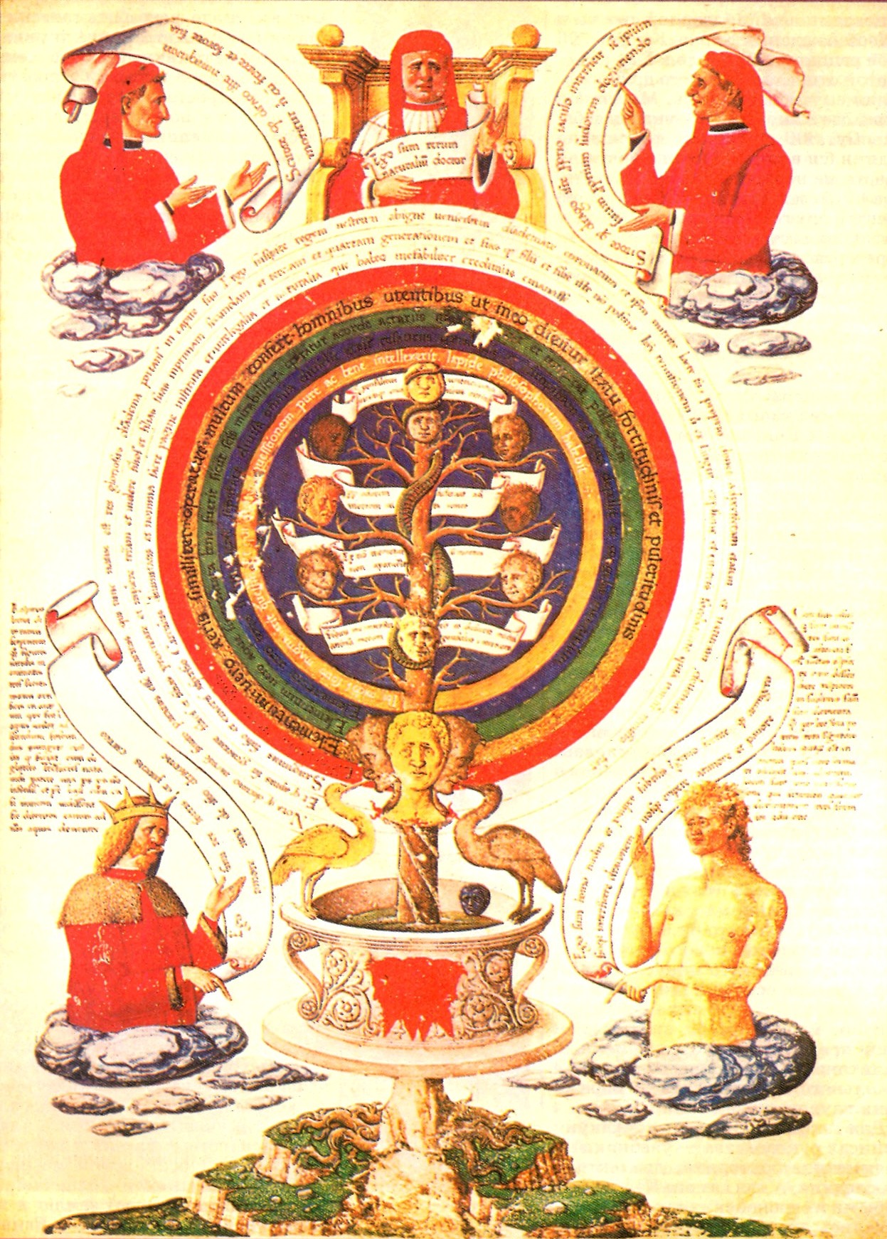 Alchemic treatise of [Ramon Llull](https://en.wikipedia.org/wiki/Ramon_Llull).
Intelligent systems find patterns and discover relations that are latent in large volumes of data.
Features of intelligent systems:
- Learning
- Adaptation
- Flexibility and robustness
- Provide explanations
- Discovery/creativity
Learning
Learning is the act of acquiring new, or modifying and reinforcing, existing knowledge, behaviors, skills, values, or preferences and may involve synthesizing different types of information.
- Construction and study of systems that can learn from data.
Adaptation
- The environment/real world is in constant change.
- The capacity to adapt implies to be able to modify what has been learn in order to cope with those modifications.
- There are many real-world cases:
- Changes in economy
- Wear of mechanic parts of a robot
- In many instances the capacity to adapt is essential to solve the problem $\rightarrow$ continuous learning.
Flexibility and robustness
- It is required to have a robust and consistent system.
- Similar inputs should generate consistent outputs.
- Self-organization
- 'Classical' approaches based on Boolean algebra and logic have limited flexibility.
Explanations
- Explanations are necessary to validate and find directions for improvement.
- It is not enough to automate the decision making process.
- In many context explanations are necessary: medicine, credit evaluation, etc.
- They are important if a human expert takes part of the decission loop.
- Machine learning can become a research tool.
Discovery/creativity
- Capacity of discovering processes and/or relations previously unknown.
- Creation of solution and artifacts.
Example: Evolving cars with genetic algorithms: http://www.boxcar2d.com/.
More formally, the machine learning can be described as: $\renewcommand{\vec}[1]{\mathbf{#1}}$
- Having a process $\mathbf{F}:\mathcal{D}\rightarrow\mathcal{I}$ that transforms a given $\vec{x}\in\mathcal{D}$ in a $\vec{y}$.
- Construct on a dataset $\Psi=\left\{\left<\vec{x}_i,\vec{y}_i\right>\right\}$ with $i=1,\ldots,N$.
- Each $\left<\vec{x}_i,\vec{y}_i\right>$ represents an input and its corresponding expected output: $\vec{y}_i=\mathbf{F}\left(\vec{x}_i\right)$.
- Optimize a model $\mathbf{M}(\vec{x};\vec{\theta})$ by adjusting its parameters $\vec{\theta}$.
- Make $\mathbf{M}()$ to be as similar as possible to $\mathbf{F}()$ by optimizing one or more error (loss) functions.
Note: Generally, $\mathcal{D}\subseteq\mathbb{R}^n$; the definition of $\mathcal{I}$ depends on the problem.
Classes of machine learning problems
- Classification: $\mathbf{F}: \mathcal{D}\rightarrow\left\{1,\ldots, k\right\}$; $\mathbf{F}(\cdot)$ defines 'categories' or 'classes' labels.
- Regression: $\mathbf{F}: \mathbb{R}^n\rightarrow\mathbb{R}$; it is necessary to predict a real-valued output instead of categories.
- Density estimation: predicit a function $p_\mathrm{model}: \mathbb{R}^n\rightarrow\mathbb{R}$, where $p_\mathrm{model}(\vec{x})$ can be interpreted as a probability density function on the set that the examples were drawn from.
- Clustering: group a set of objects in such a way that objects in the same group (cluster) are more similar to each other than to those in other groups (clusters).
- Synthesis: generate new examples that are similar to those in the training data.
Many more: times-series analysis, anomaly detection, imputation, transcription, etc.
Supervised learning
- Sometimes we can observe the pairs $\left<\vec{x}_i,\vec{y}_i\right>$:
- We can use the $\vec{y}_i$'s to provide a scalar feedback on how good is the model $\mathbf{M}(\vec{x};\vec{\theta})$.
- That feed back is known as the loss function.
- Modify parameters $\vec{\theta}$ as to improve $\mathbf{M}(\vec{x};\vec{\theta})$ $\rightarrow$ learning.
An example of a supervised problem (regression)
import random
import numpy as np
import matplotlib.pyplot as plt
plt.rc('text', usetex=True); plt.rc('font', family='serif')
plt.rc('text.latex', preamble='\\usepackage{libertine}\n\\usepackage[utf8]{inputenc}')

# numpy - pretty matrix
np.set_printoptions(precision=3, threshold=1000, edgeitems=5, linewidth=80, suppress=True)

import seaborn
seaborn.set(style='whitegrid'); seaborn.set_context('talk')

%matplotlib inline
%config InlineBackend.figure_format = 'retina'
# Fixed seed to make the results replicable - remove in real life!
random.seed(42)
x = np.arange(100)
y_real = np.sin(x/100*2*np.pi)
y_measured = y_real + (np.random.rand(100) - 0.5)/1 # simulating noise
plt.scatter(x,y_measured, marker='.', color='b', label='measured')
plt.plot(x,y_real, color='magenta', label='real')
plt.xlabel('x'); plt.ylabel('y'); plt.legend(frameon=True);

We can now learn from the dataset $\Psi=\left\{x, y_\text{measured}\right\}$.
- We are going to use a support vector regressor from
scikit-learn. - Don't get too excited, you will have to program things 'by hand'.
Training (adjusting) SVR
from sklearn.svm import SVR
clf = SVR() # using default parameters
clf.fit(x.reshape(-1, 1), y_measured)
SVR(C=1.0, cache_size=200, coef0=0.0, degree=3, epsilon=0.1, gamma='auto',
  kernel='rbf', max_iter=-1, shrinking=True, tol=0.001, verbose=False)
We can now see how our SVR models the data.
y_pred = clf.predict(x.reshape(-1, 1))
plt.scatter(x, y_measured, marker='.', color='blue', label='measured')
plt.plot(x, y_pred, color='green', label='predicted')
plt.xlabel('x'); plt.ylabel('y'); plt.legend(frameon=True);

We observe for the first time an important negative phenomenon: overfitting.

Unsupervised learning
In some cases we can just observe a series of items or values, e.g., $\Psi=\left\{\vec{x}_i\right\}$:
It is necessary to find the hidden structure of unlabeled data.
We need a measure of correctness of the model that does not requires an expected outcome.
Although, at first glance, it may look a bit awkward, this type of problem is very common.
- Related to anomaly detection, clustering, etc.
An unsupervised learning example: Clustering
Let's generate a dataset that is composed by three groups or clusters of elements, $\vec{x}\in\mathbb{R}^2$.
x_1 = np.random.randn(30,2) + (5,5)
x_2 = np.random.randn(30,2) + (10,0)
x_3 = np.random.randn(30,2) + (0,2)
plt.scatter(x_1[:,0], x_1[:,1], c='red', label='Cluster 1')
plt.scatter(x_2[:,0], x_2[:,1], c='blue', label='Cluster 2')
plt.scatter(x_3[:,0], x_3[:,1], c='green', label='Cluster 3')
plt.legend(frameon=True); plt.xlabel('$x_1$'); plt.ylabel('$x_2$');
plt.title('Three datasets');

Preparing the training dataset.
x = np.concatenate(( x_1, x_2, x_3), axis=0)
x.shape
(90, 2)
plt.scatter(x[:,0], x[:,1], c='m')
plt.title('Training dataset');

We can now try to learn what clusters are in the dataset. We are going to use the $k$-means clustering algorithm.
from sklearn.cluster import KMeans
clus = KMeans(n_clusters=3)
clus.fit(x)
KMeans(algorithm='auto', copy_x=True, init='k-means++', max_iter=300,
    n_clusters=3, n_init=10, n_jobs=1, precompute_distances='auto',
    random_state=None, tol=0.0001, verbose=0)
labels_pred = clus.predict(x)
print(labels_pred)
[2 2 2 2 2 2 2 2 2 2 2 2 2 2 2 2 2 2 2 2 2 2 2 2 2 2 2 2 2 2 1 1 1 1 1 1 1 1 1 1
 1 1 1 1 1 1 1 1 1 1 1 1 1 1 1 1 1 1 1 1 0 0 0 0 0 0 0 0 0 0 0 0 0 0 0 0 0 0 0 0
 0 0 0 0 0 0 0 0 0 0]
cm=iter(plt.cm.Set1(np.linspace(0,1,len(np.unique(labels_pred)))))
for label in np.unique(labels_pred):
    plt.scatter(x[labels_pred==label][:,0], x[labels_pred==label][:,1],
                c=next(cm), label='Pred. cluster ' +str(label+1))
plt.legend(loc='upper right', bbox_to_anchor=(1.45,1), frameon=True);
plt.xlabel('$x_1$'); plt.ylabel('$x_2$'); plt.title('Clusters predicted');

Needing to set the number of clusters can lead to problems.
clus = KMeans(n_clusters=10)
clus.fit(x)
labels_pred = clus.predict(x)
cm=iter(plt.cm.Set1(np.linspace(0,1,len(np.unique(labels_pred)))))
for label in np.unique(labels_pred):
    plt.scatter(x[labels_pred==label][:,0], x[labels_pred==label][:,1],
                c=next(cm), label='Pred. cluster ' + str(label+1))
plt.legend(loc='upper right', bbox_to_anchor=(1.45,1), frameon=True)
plt.xlabel('$x_1$'); plt.ylabel('$x_2$'); plt.title('Ten clusters predicted');

Semi-supervised learning:
- Obtaining a supervised learning dataset can be expensive.
- Some times it can be complemented with a "cheaper" unsupervised learning dataset.
- What if we first learn as much as possible from unlabeled data and then use the labeled dataset.
Reinforcement learning
- Inspired by behaviorist psychology;
- How to take actions in an environment so as to maximize some notion of cumulative reward?
- Differs from standard supervised learning in that correct input/output pairs are never presented,
- ...nor sub-optimal actions explicitly corrected.
- Involves finding a balance between exploration (of uncharted territory) and exploitation (of current knowledge).


Components of a machine learning problem/solution
- A parametrized family of functions $\mathbf{M}(\vec{x};\theta)$ describing how the learner will behave on new examples.
- What output $\mathbf{M}(\vec{x};\theta)$ will produce given some input $\vec{x}$?
- A loss function $\ell()$ describing what scalar loss $\ell(\hat{\vec{y}}, \vec{y})$ is associated with each supervised example $(x, y)$, as a function of the learner's output $\hat{\vec{y}} = f_\theta(\vec{x})$ and the target output $\vec{y}$.
- Training consists in choosing the parameters $\theta$ given some training examples $\Psi=\left\{\left<\vec{x}_i,\vec{y}_i\right>\right\}$ sampled from an unknown data generating distribution $P(X, Y)$.
Components of a machine learning problem/solution (II)
- Define a training criterion.
- Ideally: to minimize the expected loss sampled from the unknown data generating distribution.
- This is not possible because the expectation makes use of the true underlying $P()$...
- ...but we only have access to a finite number of training examples, $\Psi$.
- A training criterion usually includes an empirical average of the loss over the training set,
Components of a machine learning problem/solution (III)
- Some additional terms (called regularizers) can be added to enforce preferences over the choices of $\vec{\theta}$.
- An optimization procedure to approximately minimize the training criterion by modifying $\theta$.
Datasets and evaluation
- It is clear now that we need a dataset for training (of fitting or optimizing) the model.
- Training dataset
- We need another dataset to assess progress and compute the training criterion.
- Testing dataset
- As most ML approaches are stochastic and to contrast different approaches we need to have another dataset.
- Validation dataset
This is a cornerstone issue of machine learning and we will be comming back to it.

The machine learning flowchart
 from Scikit-learn [Choosing the right estimator](http://scikit-learn.org/stable/tutorial/machine_learning_map/index.html).
Nature-inspired machine learning
- Cellular automata
- Neural computation
- Evolutionary computation
- Swarm intelligence
- Artificial immune systems
- Membrane computing
- Amorphous computing
Final remarks
- Different classes of machine learning problems:
- Classification
- Regression
- Clustering.
- Different classes of learning scenarions:
- Supervised,
- unsupervised,
- semi-supervised, and
- reinforcement learning.
- Model, dataset, loss function, optimization.
Homework
- Read Chapter 2 of Hastie, Tibshirani and Friedman (2009) The Elements of Statistical Learning (2nd edition) Springer-Verlag.

%load_ext version_information
%version_information scipy, numpy, matplotlib
| Software | Version |
|---|---|
| Python | 3.6.1 64bit [GCC 4.2.1 Compatible Apple LLVM 6.0 (clang-600.0.57)] |
| IPython | 5.3.0 |
| OS | Darwin 16.5.0 x86_64 i386 64bit |
| scipy | 0.19.0 |
| numpy | 1.12.1 |
| matplotlib | 2.0.0 |
| Sat Apr 08 17:01:36 2017 -03 | |
# this code is here for cosmetic reasons
from IPython.core.display import HTML
from urllib.request import urlopen
HTML(urlopen('https://raw.githubusercontent.com/lmarti/jupyter_custom/master/custom.include').read().decode('utf-8'))