import sys

# install uplift library scikit-uplift and other libraries
!{sys.executable} -m pip install scikit-uplift dill catboost
📝 Load data
We are going to use a Lenta dataset from the BigTarget Hackathon hosted in summer 2020 by Lenta and Microsoft.
Lenta is a russian food retailer.
Data description
✏️ Dataset can be loaded from sklift.datasets module using fetch_lenta function.
Read more about dataset in the api docs.
This is an uplift modeling dataset containing data about Lenta's customers grociery shopping, marketing campaigns communications as treatment and store visits as target.
✏️ Major columns:
group- treatment / control flagresponse_att- binary targetCardHolder- customer idgender- customer genderage- customer age
from sklift.datasets import fetch_lenta

# returns sklearn Bunch object
# with data, target, treatment keys
# data features (pd.DataFrame), target (pd.Series), treatment (pd.Series) values
dataset = fetch_lenta()
print(f"Dataset type: {type(dataset)}\n")
print(f"Dataset features shape: {dataset.data.shape}")
print(f"Dataset target shape: {dataset.target.shape}")
print(f"Dataset treatment shape: {dataset.treatment.shape}")
Dataset type: <class 'sklearn.utils.Bunch'>

Dataset features shape: (687029, 193)
Dataset target shape: (687029,)
Dataset treatment shape: (687029,)
📝 EDA
dataset.data.head().append(dataset.data.tail())
| age | cheque_count_12m_g20 | cheque_count_12m_g21 | cheque_count_12m_g25 | cheque_count_12m_g32 | cheque_count_12m_g33 | cheque_count_12m_g38 | cheque_count_12m_g39 | cheque_count_12m_g41 | cheque_count_12m_g42 | ... | sale_sum_6m_g24 | sale_sum_6m_g25 | sale_sum_6m_g26 | sale_sum_6m_g32 | sale_sum_6m_g33 | sale_sum_6m_g44 | sale_sum_6m_g54 | stdev_days_between_visits_15d | stdev_discount_depth_15d | stdev_discount_depth_1m | |
|---|---|---|---|---|---|---|---|---|---|---|---|---|---|---|---|---|---|---|---|---|---|
| 0 | 47.0 | 3.0 | 22.0 | 19.0 | 3.0 | 28.0 | 8.0 | 7.0 | 6.0 | 1.0 | ... | 3141.25 | 356.67 | 237.25 | 283.84 | 3648.23 | 1195.37 | 535.42 | 1.7078 | 0.2798 | 0.3008 |
| 1 | 57.0 | 1.0 | 0.0 | 2.0 | 1.0 | 1.0 | 1.0 | 0.0 | 1.0 | 0.0 | ... | 113.39 | 62.69 | 58.71 | 87.01 | 179.83 | 0.00 | 122.98 | 0.0000 | 0.0000 | 0.0000 |
| 2 | 38.0 | 7.0 | 0.0 | 15.0 | 4.0 | 9.0 | 5.0 | 9.0 | 14.0 | 7.0 | ... | 1239.19 | 533.46 | 83.37 | 593.13 | 1217.43 | 1336.83 | 3709.82 | 0.0000 | NaN | 0.0803 |
| 3 | 65.0 | 6.0 | 3.0 | 25.0 | 2.0 | 10.0 | 14.0 | 11.0 | 8.0 | 1.0 | ... | 139.68 | 1849.91 | 360.40 | 175.73 | 496.73 | 172.58 | 1246.21 | 0.0000 | 0.0000 | 0.0000 |
| 4 | 61.0 | 0.0 | 1.0 | 2.0 | 0.0 | 2.0 | 1.0 | 0.0 | 3.0 | 2.0 | ... | 226.98 | 168.05 | 461.37 | 0.00 | 237.93 | 225.51 | 995.27 | 1.4142 | 0.3495 | 0.3495 |
| 687024 | 35.0 | 0.0 | 0.0 | 4.0 | 0.0 | 2.0 | 0.0 | 1.0 | 0.0 | 3.0 | ... | 550.09 | 669.33 | 111.87 | 0.00 | 330.96 | 1173.84 | 119.99 | 2.6458 | 0.3646 | 0.3282 |
| 687025 | 33.0 | 0.0 | 0.0 | 0.0 | 0.0 | 0.0 | 0.0 | 0.0 | 0.0 | 0.0 | ... | 0.00 | 0.00 | 0.00 | 0.00 | 0.00 | 0.00 | 28.01 | 0.0000 | 0.0000 | 0.0000 |
| 687026 | 36.0 | 0.0 | 0.0 | 3.0 | 0.0 | 0.0 | 0.0 | 0.0 | 1.0 | 0.0 | ... | 0.00 | 0.00 | 0.00 | 0.00 | 0.00 | 449.01 | 0.00 | 0.0000 | NaN | NaN |
| 687027 | 37.0 | 0.0 | 1.0 | 2.0 | 0.0 | 0.0 | 0.0 | 0.0 | 0.0 | 1.0 | ... | 0.00 | 46.72 | 0.00 | 0.00 | 0.00 | 0.00 | 0.00 | 0.0000 | NaN | NaN |
| 687028 | 40.0 | 0.0 | 1.0 | 0.0 | 0.0 | 2.0 | 0.0 | 0.0 | 2.0 | 2.0 | ... | 290.01 | 0.00 | 0.00 | 0.00 | 228.47 | 752.32 | 596.86 | 0.0000 | 0.0000 | 0.0000 |
10 rows × 193 columns
🤔 target share for treatment / control
import pandas as pd

pd.crosstab(dataset.treatment, dataset.target, normalize='index')
| response_att | 0 | 1 |
|---|---|---|
| group | ||
| control | 0.897421 | 0.102579 |
| test | 0.889874 | 0.110126 |
# make treatment binary
treat_dict = {
    'test': 1,
    'control': 0
}

dataset.treatment = dataset.treatment.map(treat_dict)
# fill NaNs in the categorical feature `gender`
# for CatBoostClassifier
dataset.data['gender'] = dataset.data['gender'].fillna(value='Не определен')

print(dataset.data['gender'].value_counts(dropna=False))
Ж               433448
М               243910
Не определен      9671
Name: gender, dtype: int64
✂️ train test split
- stratify by two columns: treatment and target.
Intuition: In a binary classification problem definition we stratify train set by splitting target 0/1 column. In uplift modeling we have two columns instead of one.
from sklearn.model_selection import train_test_split

stratify_cols = pd.concat([dataset.treatment, dataset.target], axis=1)

X_train, X_val, trmnt_train, trmnt_val, y_train, y_val = train_test_split(
    dataset.data,
    dataset.treatment,
    dataset.target,
    stratify=stratify_cols,
    test_size=0.3,
    random_state=42
)

print(f"Train shape: {X_train.shape}")
print(f"Validation shape: {X_val.shape}")
Train shape: (480920, 193)
Validation shape: (206109, 193)
from sklift.models import ClassTransformation
from catboost import CatBoostClassifier

estimator = CatBoostClassifier(verbose=100,
                               cat_features=['gender'],
                               random_state=42,
                               thread_count=1)

ct_model = ClassTransformation(estimator=estimator)
ct_model.fit(
    X=X_train,
    y=y_train,
    treatment=trmnt_train
)
/Users/macdrive/GoogleDrive/Проекты/Uplift/sklift-env/lib/python3.7/site-packages/ipykernel_launcher.py:4: UserWarning: It is recommended to use this approach on treatment balanced data. Current sample size is unbalanced.
  after removing the cwd from sys.path.
Learning rate set to 0.143939
0:	learn: 0.6685632	total: 1.03s	remaining: 17m 6s
100:	learn: 0.5948982	total: 1m 34s	remaining: 14m
200:	learn: 0.5907078	total: 3m 16s	remaining: 13m 3s
300:	learn: 0.5869612	total: 4m 51s	remaining: 11m 16s
400:	learn: 0.5835421	total: 6m 35s	remaining: 9m 51s
500:	learn: 0.5801981	total: 8m 31s	remaining: 8m 29s
600:	learn: 0.5769677	total: 10m 13s	remaining: 6m 47s
700:	learn: 0.5737862	total: 11m 44s	remaining: 5m
800:	learn: 0.5706947	total: 13m 37s	remaining: 3m 23s
900:	learn: 0.5677125	total: 15m 7s	remaining: 1m 39s
999:	learn: 0.5648426	total: 16m 29s	remaining: 0us
ClassTransformation(estimator=<catboost.core.CatBoostClassifier object at 0x12212bba8>)
Save model
import dill

with open("model.dill", 'wb') as f:
    dill.dump(ct_model, f)
Uplift prediction
uplift_ct = ct_model.predict(X_val)
🚀🚀🚀 Uplift metrics
🚀 uplift@k
- uplift at first k%
- usually falls between [0; 1] depending on k, model quality and data
uplift@k = target mean at k% in the treatment group - target mean at k% in the control group
How to count uplift@k:
- sort by predicted uplift
- select first k%
- count target mean in the treatment group
- count target mean in the control group
- substract the mean in the control group from the mean in the treatment group
Code parameter options:
strategy='overall'- sort by uplift treatment and control togetherstrategy='by_group'- sort by uplift treatment and control separately
from sklift.metrics import uplift_at_k

# k = 10%
k = 0.1

# strategy='overall' sort by uplift treatment and control together
uplift_overall = uplift_at_k(y_val, uplift_ct, trmnt_val, strategy='overall', k=k)

# strategy='by_group' sort by uplift treatment and control separately
uplift_bygroup = uplift_at_k(y_val, uplift_ct, trmnt_val, strategy='by_group', k=k)


print(f"uplift@{k * 100:.0f}%: {uplift_overall:.4f} (sort groups by uplift together)")
print(f"uplift@{k * 100:.0f}%: {uplift_bygroup:.4f} (sort groups by uplift separately)")
uplift@10%: 0.1467 (sort groups by uplift together)
uplift@10%: 0.1503 (sort groups by uplift separately)
🚀 uplift_by_percentile table
Count metrics for each percentile in data in descending order by uplift prediction (by rows):
n_treatment- treatment group size in the one percentilen_control- control group size in the one perentileresponse_rate_treatment- target mean in the treatment group in the one percentileresponse_rate_control- target mean in the control group in the one percentileuplift = response_rate_treatment - response_rate_controlin the one percentile
Code parameter options are:
strategy='overall'- sort by uplift treatment and control groups togetherstrategy='by_group'- sort by uplift treatment and control groups separatelytotal=True- show total metric on full datastd=True- show metrics std by row
from sklift.metrics import uplift_by_percentile

uplift_by_percentile(y_val, uplift_ct, trmnt_val,
                     strategy='overall',
                     total=True, std=True, bins=10)
| n_treatment | n_control | response_rate_treatment | response_rate_control | uplift | std_treatment | std_control | std_uplift | |
|---|---|---|---|---|---|---|---|---|
| percentile | ||||||||
| 0-10 | 12715 | 7896 | 0.366339 | 0.219605 | 0.146734 | 0.004273 | 0.004659 | 0.006321 |
| 10-20 | 15560 | 5051 | 0.214267 | 0.197783 | 0.016485 | 0.003289 | 0.005605 | 0.006499 |
| 20-30 | 15683 | 4928 | 0.149525 | 0.130682 | 0.018843 | 0.002848 | 0.004801 | 0.005582 |
| 30-40 | 15675 | 4936 | 0.111388 | 0.098663 | 0.012725 | 0.002513 | 0.004245 | 0.004933 |
| 40-50 | 15798 | 4813 | 0.082795 | 0.077914 | 0.004881 | 0.002192 | 0.003864 | 0.004442 |
| 50-60 | 15776 | 4835 | 0.062500 | 0.057911 | 0.004589 | 0.001927 | 0.003359 | 0.003873 |
| 60-70 | 15768 | 4843 | 0.051560 | 0.050176 | 0.001385 | 0.001761 | 0.003137 | 0.003597 |
| 70-80 | 15793 | 4818 | 0.042171 | 0.034869 | 0.007301 | 0.001599 | 0.002643 | 0.003089 |
| 80-90 | 15884 | 4727 | 0.035193 | 0.031521 | 0.003672 | 0.001462 | 0.002541 | 0.002932 |
| 90-100 | 16116 | 4494 | 0.039030 | 0.041611 | -0.002582 | 0.001526 | 0.002979 | 0.003347 |
| total | 154768 | 51341 | 0.110126 | 0.102569 | 0.007557 | 0.023390 | 0.037832 | 0.044615 |
from sklift.metrics import weighted_average_uplift

uplift_full_data = weighted_average_uplift(y_val, uplift_ct, trmnt_val, bins=10)
print(f"average uplift on full data: {uplift_full_data:.4f}")
average uplift on full data: 0.0189
🚀 uplift_by_percentile plot
- visualize results of
uplift_by_percentiletable
Two ways to plot:
- line plot
kind='line' - bar plot
kind='bar'
from sklift.viz import plot_uplift_by_percentile

# line plot
plot_uplift_by_percentile(y_val, uplift_ct, trmnt_val, strategy='overall', kind='line');

# bar plot
plot_uplift_by_percentile(y_val, uplift_ct, trmnt_val, strategy='overall', kind='bar');

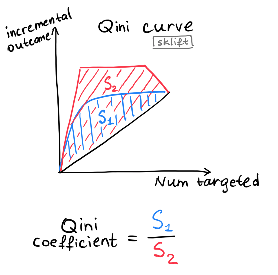
🚀 Qini curve
The curve plots the absolute incremental outcome of the treated group compared to group with no treatment.
plot Qini curve:
blue lineis areal Qini curvebased on data.red lineis anideal Qini curvebased on data. Code:perfect=Truegrey lineis arandom Qini curvebased on data
🚀 AUQC (area under Qini curve or Qini coefficient)
Qini coefficient = light blue area between the real Qini curve and the random Qini curve normalized on area between the random and the ideal line
- metric is printed at the title of the Qini curve plot
- can be called as a separate function
from sklift.viz import plot_qini_curve

# with ideal Qini curve (red line)
# perfect=True
plot_qini_curve(y_val, uplift_ct, trmnt_val, perfect=True);

# no ideal Qini curve
# only real Qini curve
# perfect=False
plot_qini_curve(y_val, uplift_ct, trmnt_val, perfect=False);

from sklift.metrics import qini_auc_score

# AUQC = area under Qini curve = Qini coefficient
auqc = qini_auc_score(y_val, uplift_ct, trmnt_val)
print(f"Qini coefficient on full data: {auqc:.4f}")
Qini coefficient on full data: 0.0695
🚀 Uplift curve
The Uplift curve plots incremental uplift.
blue lineis areal Uplift curvebased on data.red lineis anideal Uplift curvebased on data. Code:perfect=Truegrey lineis arandom Uplift curvebased on data.
🚀 AUUQ (area under uplift curve)
Area under uplift curve= blue area between the real Uplift curve and the random Uplift curve- appears at the title of the Uplift curve plot
- can be called as a separate function
from sklift.viz import plot_uplift_curve

# with ideal curve
# perfect=True
plot_uplift_curve(y_val, uplift_ct, trmnt_val, perfect=True);

# only real
# perfect=False
plot_uplift_curve(y_val, uplift_ct, trmnt_val, perfect=False);

from sklift.metrics import uplift_auc_score

# AUUQ = area under uplift curve
auuc = uplift_auc_score(y_val, uplift_ct, trmnt_val)
print(f"Uplift auc score on full data: {auuc:.4f}")
Uplift auc score on full data: 0.0422