We will need some helpers for the algebra:
load("cas_utils.sage")
var('t')
var('l g m1 m2')
xy_wsp = [('x1','x_1'),('y1','y_1'),('x2','x_2'),('y2','y_2')]

uv_wsp = [('phi','\phi'),('x','x')]

to_fun, to_var = make_symbols(xy_wsp + uv_wsp)

uv = [vars()[v] for v,lv in uv_wsp]
xy = [vars()[v] for v,lv in xy_wsp]
We introduce generalized coordinates compliant with contraints: $\varphi$, and $x$.
f(x) = sin(x)
x2u = {x1:x,x2:x+l*sin(phi),y2:-l*cos(phi)+sin(x),y1:f(x)}
showmath(x2u)
We express virtual displacement:$\delta x_1,...$ as function of virtual displacements of new coordinates: $\delta x,\delta \phi.$
for w in xy:
    vars()['d'+repr(w)+'_polar']=sum([w.subs(x2u).diff(w2)*vars()['d'+repr(w2)] for w2 in uv])
    showmath([vars()['d'+repr(w)],vars()['d'+repr(w)+'_polar']])
Now we can write d'Alembert principle:
$$\sum_{i} ( \mathbf {F}_{i} - m_i \mathbf{a}_i )\cdot \delta \mathbf r_i = 0,$$dAlemb = (m1*x1.subs(x2u).subs(to_fun).diff(t,2) )*dx1_polar + \
(m1*y1.subs(x2u).subs(to_fun).diff(t,2)+m1*g)*dy1_polar + \
(m2*x2.subs(x2u).subs(to_fun).diff(t,2) )*dx2_polar + \
(m2*y2.subs(x2u).subs(to_fun).diff(t,2)+m2*g)*dy2_polar
dAlemb = dAlemb.subs(to_var)
showmath(dAlemb.collect(dx).collect(dphi))
and derive equations of motion in new coordintes:
r1 = dAlemb.coefficient(dx)
r2 = dAlemb.coefficient(dphi)
w1,w2 =  solve([r1,r2],[xdd,phidd])[0]
showmath(w1.trig_simplify())
showmath(w2)
Special case
$m_1\to\infty$, $x=-\frac{\pi}{2}$
showmath( limit(w1.rhs(),m1=oo).subs({xdd:0,xd:0,x:-pi/2}) )
showmath( limit(w2.rhs(),m1=oo).subs({xdd:0,xd:0,x:-pi/2}).trig_reduce() )
We obtain mathematical pendulum if
showmath( limit(w1.rhs(),m1=0).trig_reduce() )
showmath( limit(w2.rhs(),m1=0).trig_reduce() )
Numerical analysis of the system
Initial conditions are four numbers: $x,\phi,\dot x,\dot \phi$.
import numpy as np
%%time
pars = {l:1,g:9.81,m1:1.,m2:1}
ode = [xd,phid,w1.rhs().subs(pars),w2.rhs().subs(pars)]
times = srange(0,10.25,0.01)
ics = [1, 0, 0, 1]
sol = desolve_odeint(ode, ics, times, [x,phi,xd,phid])
line( zip(times,sol[::1,0]),figsize=(8,2) )+\
 line( zip(times,sol[::1,1]),color='red')
line( zip(times,sol[:,0]),figsize=4 )
line( zip(np.sin(sol[:,1])+sol[:,0],-np.cos(sol[:,1])),figsize=4 )+\
 line( zip(np.sin(sol[:,1])+sol[:,0],-np.cos(sol[:,1])),figsize=4 )
Visualization
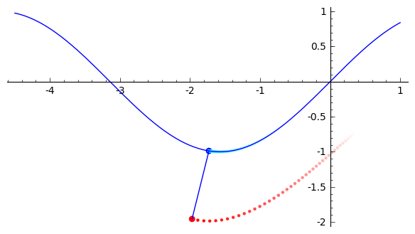
It is helpfull to write simple function displaying configuration of the system for given set of variables.
def draw_system(ith=0,l=1):
    x,phi = sol[ith,:2]
    x1,y1,x2,y2 =x, f(x),  l*sin(phi) + x,f(x)-l*cos(phi)

    p = point( (x1,y1), size=40) +\
     point( (x2,y2), size=40,color='red',figsize=3) +\
     line( [(x1,y1),(x2,y2)],aspect_ratio=1)
    n=40
    i0 = max(0,ith-n)

    trace = sum([point((l*sin(phi) + x,f(x)-l*cos(phi)),hue=(0,1-(i)/n,1)) for i,(x,phi) in enumerate(sol[ith:i0:-1,:2])])
    trace2 = sum([point((x,f(x)),hue=(.51,(i)/n,1)) for i,(x,phi) in enumerate(sol[i0:ith,:2])])

    p += trace+trace2
    var('x_')
    p += plot(f(x_),(x_,-4.5,1),figsize=6 )
    p.set_axes_range(-4.5,1,-2,1)
    p.set_aspect_ratio(1)
    return p
Let's try:
draw_system(120)
We can animate:
from IPython.display import clear_output
import time
for ith in range(0,len(sol),20):
    plt = draw_system(ith=ith,l=1)
    clear_output(wait=True)
    plt.show(figsize=3)
    time.sleep(0.021)
Alternatively one can use slider:
@interact
def _(ith=slider(range(len(sol)))):
    plt = draw_system(ith=ith,l=2)
    plt.show(figsize=6)
%%time
pars = {l:1,g:9.81,m1:1.1,m2:1}
ode = [xd,phid,w1.rhs().subs(pars),w2.rhs().subs(pars)]
times = srange(0,5000.25,0.2)
ics = [1,0,0,0]
sol = desolve_odeint(ode,ics,times,[x,phi,xd,phid])
xfft = np.fft.fft(sol[:,0])
n1 = xfft.shape[0]
plt = line(enumerate(np.abs(np.fft.fftshift(xfft))),ymax=2500,thickness=0.1)
plt.show(figsize=(8,2))
Let us check for comparison that sum of two signals with different frequencies would not cause such effect
expr = sin(1.2*t)+sin(sqrt(1.2)*t)
import numpy as np
import sympy
expr_np = np.vectorize( sympy.lambdify(t, sympy.sympify( expr ) ) )
nonchaotic = expr_np(np.linspace(0,5000,10000))
%time nonchaotic_fft = np.fft.fft(nonchaotic)
line(enumerate(nonchaotic[:234])).show(figsize=(7,2))
plt2 = line(enumerate(np.abs(np.fft.fftshift(nonchaotic_fft))),alpha=1)
plt2.show(figsize=(8,2))
Sensitivity to initial conditions
Let us compare two solution which differ by $\frac{1}{1000000}$ in initial velocity.
%%time
pars = {l:1,g:9.81,m1:1.1,m2:1}
ode = [xd,phid,w1.rhs().subs(pars),w2.rhs().subs(pars)]
times = srange(0,35.,0.1)
ics = [1,0,0,0]
sol = desolve_odeint(ode,ics,times,[x,phi,xd,phid])
ics2 = [1+1e-6,0,0,0]
sol2 = desolve_odeint(ode,ics2,times,[x,phi,xd,phid])
line(zip(times,sol[:,0]))+line(zip(times,sol2[:,0]),color='red',figsize=(6,3))
We can have a look how the error propagetes in log-scale:
line(zip(times[1:],log(abs(sol[1:,0]-sol2[1:,0]))),figsize=(6,3))
\newpage