Euler Lagrange - pendulum with oscillating support
We define Lagrange function as a difference between kinetic and potential energy:
\begin{equation} \label{eq:Lagangian} L = E_k - E_p \end{equation}Then equation of motion are given by:
\begin{equation} \label{eq:EL} \frac{d}{dt} \left (\frac{\partial L}{\partial \dot{\varphi}}\right ) - \frac{\partial L}{\partial \varphi} = 0 \end{equation}Since this formulation in invariant with respect to the change of system off coordinates, we can use it for many problems in mechanics with constraints.
System definition
Let us define a system,
load('cas_utils.sage')
var('l g w0')
xy_wsp = ['x','y']
uv_wsp = [('phi',r'\varphi')]

to_fun, to_var = make_symbols(xy_wsp, uv_wsp)
Horizontal oscillations of a support point
We parametrize the system similarily to mathematical pendulum,
\begin{eqnarray} \label{eq:parametic} x = a \sin\left(\omega t\right) + l \sin\left({\varphi}\right) \\ y = -l \cos\left({\varphi}\right) \end{eqnarray}# horizontal
var('a omega t')
x2u = {x:l*sin(phi)+a*sin(omega*t),y:-l*cos(phi)}
showmath(x2u)
Step 1: Kinetic energy
We have to write kinetic energy in terms of generalized coordinates:
\begin{equation} \label{eq:Ekin} E_k = \frac{1}{2}(\dot x^2 + \dot y^2) \end{equation}Using transformation dictionary, to generalized coordinates we have $E_k(\varphi,,\dot\varphi)$:
Ek = 1/2*sum([x_.subs(x2u).subs(to_fun).diff(t).subs(to_var)^2 for x_ in [x,y]])
Ek = Ek.trig_simplify()
showmath(Ek)
Step 2: Potential energy
Similarily we have to express potential energy:
\begin{equation} \label{eq:Ekin} E_p = g y \end{equation}as a function of $E_P(\varphi)$
Ep = g*y.subs(x2u)
showmath(Ep)
Step 3: Langranian
Now we have Lagrangian $L(\varphi,\dot\varphi)$:
L = Ek - Ep
showmath(L)
Derivation of equations of motion
Using Euler-Lagrange formulas \ref{eq:EL} we write equation of motion in generalized coordinate $\varphi$. Note, we can differentiate over $\varphi$ and $\dot\varphi$. However to perform time derivative we first replace symbols representing variables with functions (i.e. Sage symbolic functions) of time. We have to_fun dictionary which automatizes this step. Then we use symbolic differenctiation diff. After this operation we bring thhe result back to symbolic variable $\varphi$ and $\dot\varphi$ with to_var dictionary.
EL1 = L.diff(phid).subs(to_fun).diff(t).subs(to_var) - L.diff(phi)
showmath(EL1)
eq_lin = EL1.taylor(phi,0,1)
showmath(eq_lin)
var('alpha,omega0')
eq_lin2  = (eq_lin/l^2).expand().subs({a:l*alpha,g:l*omega0^2})
showmath(eq_lin2)
We see that the equations are essentially equivalent to forced harmonic oscillator. The difference might be that the effective amplitude of forcing depends on forcing frequency.
assume(g>0)
assume(omega0>0)
phi_anal = desolve((eq_lin/l^2).expand()\
                   .subs({a:l*alpha,g:l*omega0^2})\
                   .subs(to_fun).subs({l:1}),\
                   dvar=Phi,ivar=t,contrib_ode=True)
showmath(phi_anal)
showmath(eq_lin2)
Numerical integration
We can numerically compare if the linear approximation works for selected initial conditions and parameters. For this purpose we need to solve Euler-Lagrange equation for $\ddot\varphi$, and for following system od 1st order ODEs:
\begin{eqnarray} \label{eq:ode} \frac{d\varphi}{dt} &=& \dot\varphi\\ \frac{d\dot\varphi}{dt} &=& \frac{a \omega^{2} \cos\left({\varphi}\right) \sin\left(\omega t\right)}{l} - \frac{g \sin\left({\varphi}\right)}{l} \end{eqnarray}Note that we threat $\varphi$ and $\dot\varphi$ as independent variables. Since in Sage we use formulas where there are represented by different symbolic variables: phi and dphi, there will be no confusion of "dot" and derivative operator.
rhs = EL1.solve(phidd)[0].rhs()
showmath(rhs().expand())
Linear system can be derived in similar way:
rhs_lin = eq_lin.solve(phidd)[0].rhs()
showmath(rhs_lin)
pars = {l:1,g:1,a:.03,omega:1.31}
t_end = 60
w0 = sqrt(g/l).subs(pars)
Now we can plug the system of ODE into desolve_odeint solver:
ode = [phid, rhs.subs(pars)]
times = srange(0,t_end,0.1)
ics = [0.0, 0.1]
sol = desolve_odeint(ode, ics, times, [phi, phid])
line( zip(times,sol[::1,0]),figsize=(6,2), )
ode_lin = [phid, rhs_lin.subs(pars)]
times = srange(0,t_end,0.1)
ics = [0.0, 0.1]
sol_lin = desolve_odeint(ode_lin, ics, times, [phi,phid])

line( zip(times[0:],sol[0:,0]),figsize=(6,2) )\
 +line( zip(times[0:],sol_lin[0:,0]),color='red')
We see that for small oscillations the for some time. Then they diverge. One can experiment and simulate both systems for longer times to see that the divergence grows. Also larger amplitudes of driving will make them differ significantly.
Vertical oscillations
In the case of vertical oscillations of a support point, the transformation to generalized coordinates reads:
\begin{eqnarray} \label{eq:oscil_vert} x = l \sin\left({\varphi}\right)\\ y= -a \cos\left(\omega t\right) - l \cos\left({\varphi}\right), \end{eqnarray}# vertical
var('a omega t')
x2u = {x:l*sin(phi), y:-l*cos(phi)-a*cos(omega*t)}
showmath(x2u)
Let us once again calculate Lagrangian and derive symbolically equations of motion:
Ek = 1/2*sum([x_.subs(x2u).subs(to_fun).diff(t).subs(to_var)^2 for x_ in [x,y]])
Ek = Ek.trig_simplify()
Ep = g*y.subs(x2u)
L = Ek - Ep
EL1 = L.diff(phid).subs(to_fun).diff(t).subs(to_var) - L.diff(phi)
showmath(EL1)
rhs = EL1.solve(phidd)[0].rhs()
showmath( rhs.expand().collect(sin(phi)) )
Let's try to obtain a linear approximation for small $\varphi$, as in previous case:
showmath(EL1.taylor(phi,0,1) )
We see that in this case we do not obtain a harmonic oscillator. Forcing term is multiplied by $\varphi$, i.e. the linearized equation is fundamentally different.
Stable inverted pendulum
Vertical driving of a support point as a remarkable property - under some conditions the upper steady state can become a stable one.
For example for following parameters and initial condition:
pars = {l:1,a:.2,g:1,omega:10.}
w0 = sqrt(g/l).subs(pars)

ode = [phid, rhs.subs(pars) ]
times = srange(0, 60, 0.1)
ics = [pi-1e-1, .0]

sol = desolve_odeint(ode, ics, times, [phi,phid])

#plt = line( zip(times,sol[::1,0]),figsize=(8,3), ticks=[None,pi/4],\
#     tick_formatter=[None,pi],gridlines=[[],[pi.n()*i for i in range(-100,100,1)]])
plt = line( zip(times,sol[::1,0]),figsize=(6,2) )

plt.show()
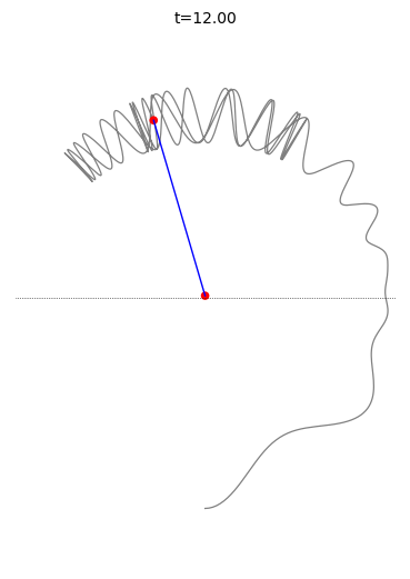
We observe that for above inital conditions the pendulum oscillates around $x=\pi$ state which is normally unstable fix point.
pendulum = [vector([x,y]).subs(x2u).subs(pars).subs({phi:phi_,t:t_})\
            for t_,phi_ in zip(times,sol[:,0])]
o_point = [vector([x,y]).subs(x2u).subs(l==0).subs(pars).subs(t==t_)\
           for t_ in times ]
#@interact
def draw_pendulum(ith = slider(0, len(pendulum)-1,1)):
    p1,p2 = pendulum[ith], o_point[ith]
    plt = line( [p1,p2],xmin=-1, xmax=1, ymin=-1.4, ymax=1.4,\
               aspect_ratio=1,figsize=2,axes=False, title='t=%0.2f'%times[ith])
    plt += points([p1,p2],color='red',size=30,gridlines=[None,[0]],\
                 figsize=3,axes=False)
    plt += line(pendulum[:ith],thickness=0.9,color='gray',zorder=-10)
    return plt
#draw_pendulum(1200).save('inverted_pend.png',figsize=8)
Time evolution of the inverted stable pendulum:
System with damping
Adding damping to the system will make inverted state an stable atractor.
$$\ddot\varphi = -2\gamma \dot\varphi + ( -\omega_0^2 - \frac{a}{l} \omega^2 \cos(\omega t))\sin(\varphi)$$var('omega,omega0,gama,t,a')
pars = {l:1,a:0.152,omega0:1,omega:14.,gama:.1}
ode = [phid,\
(-2*gama*phid+(-omega0^2-a/l*omega^2*cos(omega*t))*sin(phi)).subs(pars)]
times = srange(0,30,0.01)
ics = [0,2.1]
sol = desolve_odeint(ode,ics,times,[phi,phid])
line( zip(times,sol[::1,0]),figsize=(8,2), ticks=[None,pi/4],\
tick_formatter=[None,pi],gridlines=[[],[pi.n()*i for i in range(-100,100,1)]])
\newpage