import numpy as np
import pandas as pd
import geopandas as gpd
import seaborn as sns
import matplotlib.pyplot as plt
import matplotlib as mpl
from mpl_toolkits.axes_grid1 import make_axes_locatable
import matplotlib.patches as mpatches

plt.rcParams['savefig.facecolor'] = 'white'
%matplotlib inline
%reload_ext watermark
%watermark -v -p numpy,pandas,seaborn,matplotlib,geopandas
Python implementation: CPython
Python version       : 3.8.13
IPython version      : 8.4.0

numpy     : 1.22.4
pandas    : 1.4.2
seaborn   : 0.11.2
matplotlib: 3.5.2
geopandas : 0.9.0
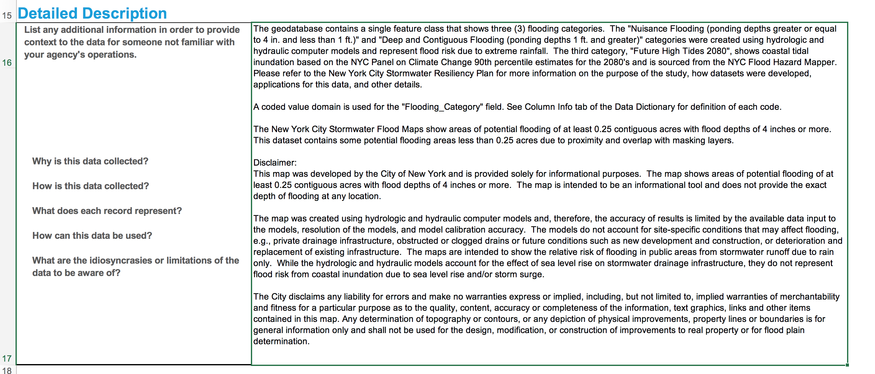
Screenshot of data description.
Source: https://data.cityofnewyork.us/City-Government/NYC-Stormwater-Flood-Map-Extreme-Flood-with-2080-S/w8eg-8ha6
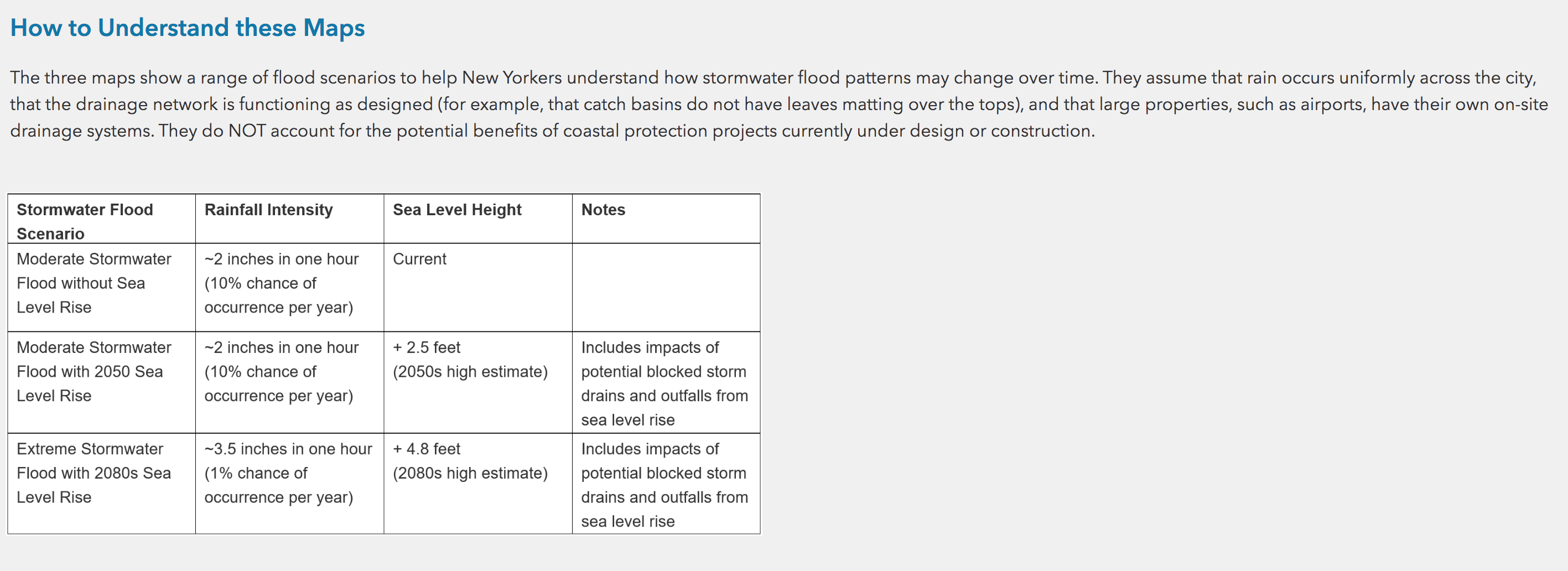
Screen shot of flood scenarios for the NYC Stormwater Flood Maps.
Source: https://experience.arcgis.com/experience/6f4cc60710dc433585790cd2b4b5dd0e
Stormwater Flood Map Layer and Geographic Boundaries
Stormwater Flood Map Layer
# read in data
gdf = gpd.read_file('data/stormwater-data.zip')

# sanity checks
print('shape of data: {}'.format(gdf.shape))
print('crs: {}'.format(gdf.crs))

# preview data
gdf.head()
shape of data: (12036, 5)
crs: epsg:2263
| Flooding_Category | flood_classification | Shape_Length | Shape_Area | geometry | |
|---|---|---|---|---|---|
| 0 | 1 | Nuisance Flooding | 1695.857677 | 27852.535494 | POLYGON Z ((916393.149 121765.469 0.000, 91640... |
| 1 | 1 | Nuisance Flooding | 1532.269198 | 18338.901687 | POLYGON Z ((917251.502 121381.664 0.000, 91725... |
| 2 | 1 | Nuisance Flooding | 2327.963831 | 32127.388341 | POLYGON Z ((916251.188 121441.271 0.000, 91625... |
| 3 | 1 | Nuisance Flooding | 3830.095703 | 48711.665246 | POLYGON Z ((917377.109 122108.195 0.000, 91739... |
| 4 | 1 | Nuisance Flooding | 4600.270710 | 65321.650657 | POLYGON Z ((918159.499 121451.773 0.000, 91814... |
NYC Boroughs
# importing borough boundaries
path = 'https://data.cityofnewyork.us/api/geospatial/tqmj-j8zm?method=export&format=Shapefile'
borough_gdf = gpd.read_file(path)
borough_gdf = borough_gdf.to_crs(2263)

# preview data
print('shape of data: {}'.format(borough_gdf.shape))
borough_gdf.head()
shape of data: (5, 5)
| boro_code | boro_name | shape_area | shape_leng | geometry | |
|---|---|---|---|---|---|
| 0 | 5.0 | Staten Island | 1.623621e+09 | 325917.353950 | MULTIPOLYGON (((970217.022 145643.332, 970227.... |
| 1 | 2.0 | Bronx | 1.187175e+09 | 463179.772813 | MULTIPOLYGON (((1012821.806 229228.265, 101278... |
| 2 | 4.0 | Queens | 3.041419e+09 | 888199.730955 | MULTIPOLYGON (((1032452.015 154469.237, 103245... |
| 3 | 1.0 | Manhattan | 6.365205e+08 | 357713.308660 | MULTIPOLYGON (((981219.056 188655.316, 980940.... |
| 4 | 3.0 | Brooklyn | 1.934138e+09 | 728148.532410 | MULTIPOLYGON (((1022227.320 152028.146, 102207... |
Neigborhood Tabulation Area (NTA)
# importing neighborhood boundaries
path = 'https://data.cityofnewyork.us/api/geospatial/9nt8-h7nd?accessType=DOWNLOAD&method=export&format=Shapefile'
nta_gdf = gpd.read_file(path)
nta_gdf = nta_gdf.to_crs(2263)

# preview data
print('shape of data: {}'.format(nta_gdf.shape))
nta_gdf.head()
shape of data: (262, 12)
| borocode | boroname | countyfips | nta2020 | ntaname | ntaabbrev | ntatype | cdta2020 | cdtaname | shape_leng | shape_area | geometry | |
|---|---|---|---|---|---|---|---|---|---|---|---|---|
| 0 | 1.0 | Manhattan | 061 | MN6491 | Central Park | CntrlPk | 9 | MN64 | MN64 Central Park (JIA 64 Equivalent) | 32721.097429 | 3.831238e+07 | POLYGON ((997412.248 230101.816, 997436.269 23... |
| 1 | 1.0 | Manhattan | 061 | MN0401 | Chelsea-Hudson Yards | Chls_HdsYd | 0 | MN04 | MN04 Chelsea-Hell's Kitchen (CD 4 Approximation) | 40095.235570 | 2.967175e+07 | POLYGON ((983031.177 217138.506, 983640.320 21... |
| 2 | 1.0 | Manhattan | 061 | MN0301 | Chinatown-Two Bridges | Chntwn | 0 | MN03 | MN03 Lower East Side-Chinatown (CD 3 Equivalent) | 16464.371337 | 1.154263e+07 | POLYGON ((987256.457 200392.989, 987090.306 19... |
| 3 | 1.0 | Manhattan | 061 | MN1102 | East Harlem (North) | EstHrlm_N | 0 | MN11 | MN11 East Harlem (CD 11 Equivalent) | 28710.999462 | 2.610451e+07 | MULTIPOLYGON (((1004410.678 229781.419, 100436... |
| 4 | 1.0 | Manhattan | 061 | MN1101 | East Harlem (South) | EstHrlm_S | 0 | MN11 | MN11 East Harlem (CD 11 Equivalent) | 18682.264948 | 1.665394e+07 | POLYGON ((1000577.175 228028.553, 1001238.138 ... |
I like having the borough boundaries as general map boundaries for New York City. However, I like calculating statistics at the Neighborhood Tabulation Area (NTA) level.
Exploratory Stormwater Flood Maps
fig, ax = plt.subplots(figsize=(8, 8))

gdf.plot(ax=ax)

borough_gdf.plot(
    ax=ax,
    facecolor='none',
    edgecolor='black',
    zorder=1
)

plt.title('NYC Stormwater Flood Map\nExtreme Flood With 2080 Sea Level Rise', fontsize=15)
plt.axis('off')
plt.tight_layout()
Figure xx: NYC Stormwater Flood Map Extreme Flood With 2080 Sea Level Rise.
fig, ax = plt.subplots(figsize=(8, 8))

patches = []
colors = ['tab:cyan', 'blue', 'tab:orange']
classifications = gdf['flood_classification'].unique()

for label, color in zip(classifications, colors):

    (gdf
     .loc[gdf['flood_classification'].isin([label])]
     .plot(color=color, ax=ax)
    )

    patches.append(mpatches.Patch(color=color, label=label))

borough_gdf.plot(
    ax=ax,
    facecolor='none',
    edgecolor='black',
    zorder=1
)

plt.legend(
    title='',
    handles=patches,
    fontsize='12',
    loc=2
)

title = 'NYC Stormwater Flood Map - Extreme Flood\nWith 2080 Sea Level Rise by Flood Classification'
plt.title(title, fontsize=14)
plt.axis('off')
plt.tight_layout()

# save as repo cover photo
plt.savefig('figures/cover-map.png', dpi=250, bbox_inches='tight')
Figure xx: NYC Stormwater Flood Map Extreme Flood With 2080 Sea Level Rise by Flood Classification.
Summary Flood Risk Statistics by Neighborhood Tabulation Area
Percent of Buildings Flooded
Neighborhoods with at least 80 buildings.
ls data/
buildings-hazard.csv      hourly-precipitation.csv  stormwater-data-source/
daily-precipitation.csv   nta-hazard.csv            stormwater-data.zip
# percent of buildings flooded by neighborhood
path = 'data/buildings-hazard.csv'
df = pd.read_csv(path)

# preview data
print('shape of data: {}'.format(df.shape))
df.head()
shape of data: (491, 8)
| nta2020 | building_count | flood_classification | flooded_count | flooded_perc | ntaname | boroname | ntaname_boro | |
|---|---|---|---|---|---|---|---|---|
| 0 | QN1001 | 23685 | Deep and Contiguous Flooding | 1812 | 7.65 | South Ozone Park | Queens | South Ozone Park, Queens |
| 1 | QN1001 | 23685 | Nuisance Flooding | 1285 | 5.43 | South Ozone Park | Queens | South Ozone Park, Queens |
| 2 | QN1303 | 19817 | Nuisance Flooding | 1691 | 8.53 | Queens Village | Queens | Queens Village, Queens |
| 3 | QN1303 | 19817 | Deep and Contiguous Flooding | 1231 | 6.21 | Queens Village | Queens | Queens Village, Queens |
| 4 | QN1205 | 18814 | Deep and Contiguous Flooding | 2304 | 12.25 | St. Albans | Queens | St. Albans, Queens |
# summary statistics of percent of buildings flooded by neigborhood
(df
 .groupby(by='flood_classification')['flooded_perc']
 .describe()
)
| count | mean | std | min | 25% | 50% | 75% | max | |
|---|---|---|---|---|---|---|---|---|
| flood_classification | ||||||||
| Deep and Contiguous Flooding | 197.0 | 6.540254 | 5.315112 | 0.05 | 2.81 | 5.28 | 9.160 | 34.34 |
| Future High Tides 2080 | 83.0 | 5.025060 | 12.944060 | 0.01 | 0.15 | 0.45 | 2.085 | 76.47 |
| Nuisance Flooding | 203.0 | 6.085665 | 3.797289 | 0.32 | 3.56 | 5.34 | 7.480 | 25.38 |
Table xx: Summary statistics of percent of buildings flooded by Neighborhood Tabulation Area (NTA).
Percent of Buildings Flooded: Deep and Contiguous Flooding
cols = [
    'nta2020', 'ntaname_boro', 'building_count',
    'flood_classification', 'flooded_count', 'flooded_perc'
]

classification = 'Deep and Contiguous Flooding'

# join nta derived flood data to nta geodataframe
merged_gdf = nta_gdf.merge(
    df.loc[df['flood_classification'] == classification, cols],
    on='nta2020',
    how='left'
)

cols = ['building_count', 'flooded_count', 'flooded_perc']
for col in cols:
    merged_gdf[col] = merged_gdf[col].fillna(0)

print('shape of data: {}'.format(merged_gdf.shape))
merged_gdf.head()
shape of data: (262, 17)
| borocode | boroname | countyfips | nta2020 | ntaname | ntaabbrev | ntatype | cdta2020 | cdtaname | shape_leng | shape_area | geometry | ntaname_boro | building_count | flood_classification | flooded_count | flooded_perc | |
|---|---|---|---|---|---|---|---|---|---|---|---|---|---|---|---|---|---|
| 0 | 1.0 | Manhattan | 061 | MN6491 | Central Park | CntrlPk | 9 | MN64 | MN64 Central Park (JIA 64 Equivalent) | 32721.097429 | 3.831238e+07 | POLYGON ((997412.248 230101.816, 997436.269 23... | NaN | 0.0 | NaN | 0.0 | 0.00 |
| 1 | 1.0 | Manhattan | 061 | MN0401 | Chelsea-Hudson Yards | Chls_HdsYd | 0 | MN04 | MN04 Chelsea-Hell's Kitchen (CD 4 Approximation) | 40095.235570 | 2.967175e+07 | POLYGON ((983031.177 217138.506, 983640.320 21... | Chelsea-Hudson Yards, Manhattan | 2092.0 | Deep and Contiguous Flooding | 121.0 | 5.78 |
| 2 | 1.0 | Manhattan | 061 | MN0301 | Chinatown-Two Bridges | Chntwn | 0 | MN03 | MN03 Lower East Side-Chinatown (CD 3 Equivalent) | 16464.371337 | 1.154263e+07 | POLYGON ((987256.457 200392.989, 987090.306 19... | Chinatown-Two Bridges, Manhattan | 1126.0 | Deep and Contiguous Flooding | 7.0 | 0.62 |
| 3 | 1.0 | Manhattan | 061 | MN1102 | East Harlem (North) | EstHrlm_N | 0 | MN11 | MN11 East Harlem (CD 11 Equivalent) | 28710.999462 | 2.610451e+07 | MULTIPOLYGON (((1004410.678 229781.419, 100436... | East Harlem (North), Manhattan | 2002.0 | Deep and Contiguous Flooding | 72.0 | 3.60 |
| 4 | 1.0 | Manhattan | 061 | MN1101 | East Harlem (South) | EstHrlm_S | 0 | MN11 | MN11 East Harlem (CD 11 Equivalent) | 18682.264948 | 1.665394e+07 | POLYGON ((1000577.175 228028.553, 1001238.138 ... | East Harlem (South), Manhattan | 1033.0 | Deep and Contiguous Flooding | 156.0 | 15.10 |
(merged_gdf
 .sort_values(by='flooded_perc', ascending=False)
 .loc[:, ['ntaname_boro', 'building_count', 'flooded_count', 'flooded_perc']]
 .astype({'building_count':'int', 'flooded_count':'int'})
 .head(20)
 .reset_index(drop=True)
 .set_index([pd.Series(range(1, 21))])
)
| ntaname_boro | building_count | flooded_count | flooded_perc | |
|---|---|---|---|---|
| 1 | Pelham Parkway-Van Nest, Bronx | 2190 | 752 | 34.34 |
| 2 | Gravesend (South), Brooklyn | 3175 | 888 | 27.97 |
| 3 | Ozone Park (North), Queens | 5245 | 1345 | 25.64 |
| 4 | Old Astoria-Hallets Point, Queens | 1609 | 399 | 24.80 |
| 5 | East New York-New Lots, Brooklyn | 6358 | 1332 | 20.95 |
| 6 | Westchester Square, Bronx | 2031 | 417 | 20.53 |
| 7 | Parkchester, Bronx | 571 | 108 | 18.91 |
| 8 | South Williamsburg, Brooklyn | 2284 | 418 | 18.30 |
| 9 | Tribeca-Civic Center, Manhattan | 911 | 162 | 17.78 |
| 10 | Inwood, Manhattan | 604 | 93 | 15.40 |
| 11 | East Harlem (South), Manhattan | 1033 | 156 | 15.10 |
| 12 | Baisley Park, Queens | 11903 | 1658 | 13.93 |
| 13 | Bedford-Stuyvesant (West), Brooklyn | 7564 | 1047 | 13.84 |
| 14 | East New York-City Line, Brooklyn | 4371 | 604 | 13.82 |
| 15 | Hollis, Queens | 6899 | 939 | 13.61 |
| 16 | Soundview-Bruckner-Bronx River, Bronx | 4445 | 597 | 13.43 |
| 17 | Springfield Gardens (South)-Brookville, Queens | 5505 | 738 | 13.41 |
| 18 | East Midtown-Turtle Bay, Manhattan | 1111 | 140 | 12.60 |
| 19 | Greenpoint, Brooklyn | 5162 | 633 | 12.26 |
| 20 | St. Albans, Queens | 18814 | 2304 | 12.25 |
Table xx: Top 20 percent of flooded buildings from Deep and Contiguous Flooding by Neighborhood Tablulation Area (NTA).
fig, ax = plt.subplots(figsize=(8, 6))

label = 'Deep and Contiguous Flooding'

data = (
    merged_gdf
    .sort_values(by='flooded_perc', ascending=False)
    .loc[:, ['ntaname_boro', 'building_count', 'flooded_count', 'flooded_perc']]
    .head(20)
)

sns.barplot(
    data=data,
    y='ntaname_boro',
    x='flooded_perc',
    color='C0',
    ax=ax
)

patches = [mpatches.Patch(label=label)]
plt.legend(handles=patches, loc=4, fontsize=10)

plt.title('NYC Stormwater Flood Map - Extreme Flood\n\
Percent of Flooded Buildings by Neighborhood', fontsize=12)
plt.xlabel('Percent of Flooded Buildings')
plt.ylabel('Neighborhood')
plt.tight_layout()
Figure xx: Top 20 percent of flooded buildings from Deep and Contiguous Flooding by Neighborhood Tablulation Area (NTA).
fig, ax = plt.subplots(figsize=(8, 8))

divider = make_axes_locatable(ax)
cax = divider.append_axes("right", size="5%", pad=0.1)
cmap = plt.cm.Blues
norm = mpl.colors.BoundaryNorm([0, 5, 10, 15, 20, 40], cmap.N)

merged_gdf.plot(
    column='flooded_perc',
    legend=True,
    cmap=cmap,
    norm=norm,
    ax=ax,
    cax=cax,
)

nta_gdf.plot(
    ax=ax,
    zorder=1,
    facecolor='None',
    linewidth=.4,
)

title = "NYC's Stormwater Flood Map - Extreme Flood Scenario"
sup_title = 'Percent of Buildings Flooded by Deep and Contiguous Flooding by Neighborhood'
ax.set_title('{}\n{}'.format(title, sup_title))

ax.axis('off')
plt.tight_layout()
plt.savefig('figures/deep-flood-buildings-perc.png', dpi=250, bbox_inches='tight')
Figure xx: Percent of buildings flooded from Deep and Contiguous Flooding by Neighborhood Tabulation Area (NTA).
boros = merged_gdf['boroname'].unique()

for boro in boros:
    fig, ax = plt.subplots(figsize=(8, 8))

    divider = make_axes_locatable(ax)
    cax = divider.append_axes("right", size="5%", pad=0.1)
    cmap = plt.cm.Blues

    (merged_gdf
     .loc[merged_gdf['boroname'] == boro]
     .plot(
        column='flooded_perc',
        legend=True,
        cmap=cmap,
        ax=ax,
        cax=cax)
    )

    (nta_gdf
     .loc[nta_gdf['boroname'] == boro]
     .plot(
        ax=ax,
        zorder=1,
        facecolor='None',
        linewidth=.4)
    )

    title = "NYC's Stormwater Flood Map - Extreme Flood Scenario"
    sup_title = 'Percent of Buildings Flooded by Deep and Contiguous Flooding in {}'.format(boro)
    ax.set_title('{}\n{}'.format(title, sup_title))

    ax.axis('off')
    plt.tight_layout()
Figure xx: Percent of buildings flooded from Deep and Contiguous Flooding by Neighborhood Tabulation Area (NTA) for boroughs in New York City.
Percent of Buildings Flooded: Future High Tides 2080
cols = [
    'nta2020', 'ntaname_boro', 'building_count',
    'flood_classification', 'flooded_count', 'flooded_perc'
]

classification = 'Future High Tides 2080'

merged_gdf = nta_gdf.merge(
    df.loc[df['flood_classification'] == classification, cols],
    on='nta2020',
    how='left'
)

cols = ['building_count', 'flooded_count', 'flooded_perc']
for col in cols:
    merged_gdf[col] = merged_gdf[col].fillna(0)

print('shape of data: {}'.format(merged_gdf.shape))
merged_gdf.head()
shape of data: (262, 17)
| borocode | boroname | countyfips | nta2020 | ntaname | ntaabbrev | ntatype | cdta2020 | cdtaname | shape_leng | shape_area | geometry | ntaname_boro | building_count | flood_classification | flooded_count | flooded_perc | |
|---|---|---|---|---|---|---|---|---|---|---|---|---|---|---|---|---|---|
| 0 | 1.0 | Manhattan | 061 | MN6491 | Central Park | CntrlPk | 9 | MN64 | MN64 Central Park (JIA 64 Equivalent) | 32721.097429 | 3.831238e+07 | POLYGON ((997412.248 230101.816, 997436.269 23... | NaN | 0.0 | NaN | 0.0 | 0.00 |
| 1 | 1.0 | Manhattan | 061 | MN0401 | Chelsea-Hudson Yards | Chls_HdsYd | 0 | MN04 | MN04 Chelsea-Hell's Kitchen (CD 4 Approximation) | 40095.235570 | 2.967175e+07 | POLYGON ((983031.177 217138.506, 983640.320 21... | Chelsea-Hudson Yards, Manhattan | 2092.0 | Future High Tides 2080 | 72.0 | 3.44 |
| 2 | 1.0 | Manhattan | 061 | MN0301 | Chinatown-Two Bridges | Chntwn | 0 | MN03 | MN03 Lower East Side-Chinatown (CD 3 Equivalent) | 16464.371337 | 1.154263e+07 | POLYGON ((987256.457 200392.989, 987090.306 19... | Chinatown-Two Bridges, Manhattan | 1126.0 | Future High Tides 2080 | 8.0 | 0.71 |
| 3 | 1.0 | Manhattan | 061 | MN1102 | East Harlem (North) | EstHrlm_N | 0 | MN11 | MN11 East Harlem (CD 11 Equivalent) | 28710.999462 | 2.610451e+07 | MULTIPOLYGON (((1004410.678 229781.419, 100436... | East Harlem (North), Manhattan | 2002.0 | Future High Tides 2080 | 10.0 | 0.50 |
| 4 | 1.0 | Manhattan | 061 | MN1101 | East Harlem (South) | EstHrlm_S | 0 | MN11 | MN11 East Harlem (CD 11 Equivalent) | 18682.264948 | 1.665394e+07 | POLYGON ((1000577.175 228028.553, 1001238.138 ... | East Harlem (South), Manhattan | 1033.0 | Future High Tides 2080 | 4.0 | 0.39 |
(merged_gdf
 .sort_values(by='flooded_perc', ascending=False)
 .loc[:, ['ntaname_boro', 'building_count', 'flooded_count', 'flooded_perc']]
 .astype({'building_count':'int', 'flooded_count':'int'})
 .head(20)
 .reset_index(drop=True)
 .set_index([pd.Series(range(1, 21))])
)
| ntaname_boro | building_count | flooded_count | flooded_perc | |
|---|---|---|---|---|
| 1 | Rockaway Beach-Arverne-Edgemere, Queens | 4454 | 3406 | 76.47 |
| 2 | Breezy Point-Belle Harbor-Rockaway Park-Broad ... | 9424 | 6124 | 64.98 |
| 3 | Coney Island-Sea Gate, Brooklyn | 3358 | 1162 | 34.60 |
| 4 | Howard Beach-Lindenwood, Queens | 6870 | 2064 | 30.04 |
| 5 | Brighton Beach, Brooklyn | 2072 | 620 | 29.92 |
| 6 | Far Rockaway-Bayswater, Queens | 6786 | 1817 | 26.78 |
| 7 | Financial District-Battery Park City, Manhattan | 635 | 170 | 26.77 |
| 8 | Stuyvesant Town-Peter Cooper Village, Manhattan | 81 | 18 | 22.22 |
| 9 | Jacob Riis Park-Fort Tilden-Breezy Point Tip, ... | 164 | 31 | 18.90 |
| 10 | Sheepshead Bay-Manhattan Beach-Gerritsen Beach... | 11282 | 1857 | 16.46 |
| 11 | Flushing Meadows-Corona Park, Queens | 163 | 12 | 7.36 |
| 12 | Rosedale, Queens | 7665 | 383 | 5.00 |
| 13 | Long Island City-Hunters Point, Queens | 1305 | 64 | 4.90 |
| 14 | Carroll Gardens-Cobble Hill-Gowanus-Red Hook, ... | 7469 | 347 | 4.65 |
| 15 | Chelsea-Hudson Yards, Manhattan | 2092 | 72 | 3.44 |
| 16 | Barren Island-Floyd Bennett Field, Brooklyn | 89 | 3 | 3.37 |
| 17 | Springfield Gardens (South)-Brookville, Queens | 5505 | 181 | 3.29 |
| 18 | Throgs Neck-Schuylerville, Bronx | 11218 | 338 | 3.01 |
| 19 | New Dorp-Midland Beach, Staten Island | 10041 | 292 | 2.91 |
| 20 | Oakwood-Richmondtown, Staten Island | 6751 | 187 | 2.77 |
Table xx: Top 20 percent of buildings flooded from Future High Tides 2080 by Neighborhood Tabulation Area (NTA).
fig, ax = plt.subplots(figsize=(8, 6))

label = 'Future High Tides 2080'

data = (
    merged_gdf
    .sort_values(by='flooded_perc', ascending=False)
    .loc[:, ['ntaname_boro', 'building_count', 'flooded_count', 'flooded_perc']]
    .head(20)
)

sns.barplot(
    data=data,
    y='ntaname_boro',
    x='flooded_perc',
    color='C0',
    ax=ax
)

patches = [mpatches.Patch(label=label)]
plt.legend(handles=patches, loc=4, fontsize=10)

plt.title('NYC Stormwater Flood Map - Extreme Flood\n\
Percent of Flooded Buildings by Neighborhood', fontsize=12)
plt.xlabel('Percent of Flooded Buildings')
plt.ylabel('Neighborhood')
plt.tight_layout()
Figuree xx: Top 20 percent of buildings flooded from Future High Tides 2080 by Neighborhood Tabulation Area (NTA).
fig, ax = plt.subplots(figsize=(8, 8))

divider = make_axes_locatable(ax)
cax = divider.append_axes("right", size="5%", pad=0.1)
cmap = plt.cm.Blues
norm = mpl.colors.BoundaryNorm([0, 2.5, 5, 10, 20, 40, 80], cmap.N)

merged_gdf.plot(
    column='flooded_perc',
    legend=True,
    cmap=cmap,
    norm=norm,
    ax=ax,
    cax=cax,
)

nta_gdf.plot(
    ax=ax,
    zorder=1,
    facecolor='None',
    linewidth=.5,
)

title = "NYC's Stormwater Flood Map - Extreme Flood Scenario"
sup_title = 'Percent of Buildings Flooded by Future High Tides 2080 by Neighborhood'
ax.set_title('{}\n{}'.format(title, sup_title))

ax.axis('off')
plt.tight_layout()
plt.savefig('figures/high-tide-buildings-perc.png', dpi=250, bbox_inches='tight')
Figure xx: Percent of buildings flooded from Future High Tides 2080 by Neighborhood Tabulation Area (NTA).
boros = merged_gdf['boroname'].unique()

for boro in boros:
    fig, ax = plt.subplots(figsize=(8, 8))

    divider = make_axes_locatable(ax)
    cax = divider.append_axes("right", size="5%", pad=0.1)
    cmap = plt.cm.Blues

    (merged_gdf
     .loc[merged_gdf['boroname'] == boro]
     .plot(
        column='flooded_perc',
        legend=True,
        cmap=cmap,
        ax=ax,
        cax=cax)
    )

    (nta_gdf
     .loc[nta_gdf['boroname'] == boro]
     .plot(
        ax=ax,
        zorder=1,
        facecolor='None',
        linewidth=.4)
    )

    title = "NYC's Stormwater Flood Map - Extreme Flood Scenario"
    sup_title = 'Percent of Buildings Flooded by Future High Tides 2080 by Neighborhood in {}'.format(boro)
    ax.set_title('{}\n{}'.format(title, sup_title))

    ax.axis('off')
    plt.tight_layout()
Figure xx: Percent of buildings flooded from Future High Tides 2080 by Neighborhood Tabulation Area (NTA) for boroughs in New York City.
Percent of Area Flooded
ls data/
buildings-hazard.csv      hourly-precipitation.csv  stormwater-data-source/
daily-precipitation.csv   nta-hazard.csv            stormwater-data.zip
# percent of area flooded by neigborhood
path = 'data/nta-hazard.csv'
df = pd.read_csv(path)

print('shape of data: {}'.format(df.shape))
df.head()
shape of data: (620, 8)
| nta2020 | shape_area | flood_classification | flooded_area | flooded_area_perc | ntaname | boroname | ntaname_boro | |
|---|---|---|---|---|---|---|---|---|
| 0 | BK0101 | 3.532121e+07 | Deep and Contiguous Flooding | 1.790620e+06 | 5.07 | Greenpoint | Brooklyn | Greenpoint, Brooklyn |
| 1 | BK0101 | 3.532121e+07 | Future High Tides 2080 | 2.038655e+06 | 5.77 | Greenpoint | Brooklyn | Greenpoint, Brooklyn |
| 2 | BK0101 | 3.532121e+07 | Nuisance Flooding | 1.307740e+06 | 3.70 | Greenpoint | Brooklyn | Greenpoint, Brooklyn |
| 3 | BK0102 | 2.885436e+07 | Deep and Contiguous Flooding | 1.706097e+06 | 5.91 | Williamsburg | Brooklyn | Williamsburg, Brooklyn |
| 4 | BK0102 | 2.885436e+07 | Future High Tides 2080 | 7.384257e+05 | 2.56 | Williamsburg | Brooklyn | Williamsburg, Brooklyn |
# summary statistics of percent of area flooded by neigborhood
(df
 .groupby(by='flood_classification')['flooded_area_perc']
 .describe()
)
| count | mean | std | min | 25% | 50% | 75% | max | |
|---|---|---|---|---|---|---|---|---|
| flood_classification | ||||||||
| Deep and Contiguous Flooding | 240.0 | 3.284000 | 2.737847 | 0.01 | 1.1325 | 2.460 | 5.1825 | 14.30 |
| Future High Tides 2080 | 132.0 | 5.445758 | 9.065596 | 0.00 | 0.5550 | 1.895 | 5.4325 | 56.21 |
| Nuisance Flooding | 248.0 | 3.565484 | 2.510365 | 0.02 | 1.6100 | 3.285 | 5.1100 | 11.47 |
Table xx: Summary statistics of percent of area flooded by Neighborhood Tabulation Area (NTA).
Percent of Area Flooded: Deep and Contiguous Flooding
cols = [
    'nta2020', 'ntaname_boro',
    'flood_classification', 'flooded_area', 'flooded_area_perc'
]

classification = 'Deep and Contiguous Flooding'

merged_gdf = nta_gdf.merge(
    df.loc[df['flood_classification'] == classification, cols],
    on='nta2020',
    how='left'
)

cols = ['shape_area', 'flooded_area', 'flooded_area_perc']
for col in cols:
    merged_gdf[col] = merged_gdf[col].fillna(0)

print('shape of data: {}'.format(merged_gdf.shape))
merged_gdf.head()
shape of data: (262, 16)
| borocode | boroname | countyfips | nta2020 | ntaname | ntaabbrev | ntatype | cdta2020 | cdtaname | shape_leng | shape_area | geometry | ntaname_boro | flood_classification | flooded_area | flooded_area_perc | |
|---|---|---|---|---|---|---|---|---|---|---|---|---|---|---|---|---|
| 0 | 1.0 | Manhattan | 061 | MN6491 | Central Park | CntrlPk | 9 | MN64 | MN64 Central Park (JIA 64 Equivalent) | 32721.097429 | 3.831238e+07 | POLYGON ((997412.248 230101.816, 997436.269 23... | NaN | NaN | 0.000000 | 0.00 |
| 1 | 1.0 | Manhattan | 061 | MN0401 | Chelsea-Hudson Yards | Chls_HdsYd | 0 | MN04 | MN04 Chelsea-Hell's Kitchen (CD 4 Approximation) | 40095.235570 | 2.967175e+07 | POLYGON ((983031.177 217138.506, 983640.320 21... | Chelsea-Hudson Yards, Manhattan | Deep and Contiguous Flooding | 625930.867140 | 2.11 |
| 2 | 1.0 | Manhattan | 061 | MN0301 | Chinatown-Two Bridges | Chntwn | 0 | MN03 | MN03 Lower East Side-Chinatown (CD 3 Equivalent) | 16464.371337 | 1.154263e+07 | POLYGON ((987256.457 200392.989, 987090.306 19... | Chinatown-Two Bridges, Manhattan | Deep and Contiguous Flooding | 77539.916379 | 0.67 |
| 3 | 1.0 | Manhattan | 061 | MN1102 | East Harlem (North) | EstHrlm_N | 0 | MN11 | MN11 East Harlem (CD 11 Equivalent) | 28710.999462 | 2.610451e+07 | MULTIPOLYGON (((1004410.678 229781.419, 100436... | East Harlem (North), Manhattan | Deep and Contiguous Flooding | 371509.986399 | 1.42 |
| 4 | 1.0 | Manhattan | 061 | MN1101 | East Harlem (South) | EstHrlm_S | 0 | MN11 | MN11 East Harlem (CD 11 Equivalent) | 18682.264948 | 1.665394e+07 | POLYGON ((1000577.175 228028.553, 1001238.138 ... | East Harlem (South), Manhattan | Deep and Contiguous Flooding | 622475.411398 | 3.74 |
(merged_gdf
 .sort_values(by='flooded_area_perc', ascending=False)
 .loc[:, ['ntaname_boro', 'shape_area', 'flooded_area', 'flooded_area_perc']]
 .set_index('ntaname_boro')
 .div({'shape_area':43560, 'flooded_area':43560, 'flooded_area_perc':1})
 .astype({'shape_area':int, 'flooded_area':int})
 .rename(columns={'shape_area':'shape_area_acre', 'flooded_area':'flooded_area_acre'})
 .head(20)
 .reset_index(drop=False)
 .set_index([pd.Series(range(1, 21))])
)
| ntaname_boro | shape_area_acre | flooded_area_acre | flooded_area_perc | |
|---|---|---|---|---|
| 1 | South Williamsburg, Brooklyn | 349 | 49 | 14.30 |
| 2 | Gravesend (South), Brooklyn | 593 | 78 | 13.17 |
| 3 | Ozone Park (North), Queens | 415 | 50 | 12.17 |
| 4 | Fresh Meadows-Utopia, Queens | 762 | 80 | 10.57 |
| 5 | East New York-New Lots, Brooklyn | 1066 | 104 | 9.83 |
| 6 | South Jamaica, Queens | 869 | 83 | 9.59 |
| 7 | Hollis, Queens | 561 | 53 | 9.48 |
| 8 | Corona, Queens | 551 | 50 | 9.21 |
| 9 | Old Astoria-Hallets Point, Queens | 254 | 23 | 9.16 |
| 10 | Tribeca-Civic Center, Manhattan | 311 | 27 | 8.98 |
| 11 | Baisley Park, Queens | 1100 | 95 | 8.67 |
| 12 | Bushwick (East), Brooklyn | 641 | 54 | 8.49 |
| 13 | New Dorp-Midland Beach, Staten Island | 1427 | 119 | 8.40 |
| 14 | St. Albans, Queens | 1705 | 141 | 8.32 |
| 15 | Gravesend (West), Brooklyn | 776 | 64 | 8.28 |
| 16 | Flatlands, Brooklyn | 1247 | 97 | 7.83 |
| 17 | Jamaica, Queens | 1075 | 83 | 7.78 |
| 18 | SoHo-Little Italy-Hudson Square, Manhattan | 296 | 23 | 7.78 |
| 19 | Bedford-Stuyvesant (East), Brooklyn | 947 | 71 | 7.54 |
| 20 | Sunnyside Yards (North), Queens | 103 | 7 | 7.45 |
Table xx: Top 20 percent of flooded area from Deep and Contiguous Flooding by Neighborhood Tablulation Area (NTA).
fig, ax = plt.subplots(figsize=(8, 6))

label = 'Deep and Contiguous Flooding'

data = (
    merged_gdf
    .sort_values(by='flooded_area_perc', ascending=False)
    .loc[:, ['ntaname_boro', 'flooded_area', 'flooded_area_perc']]
    .head(20)
)

sns.barplot(
    data=data,
    y='ntaname_boro',
    x='flooded_area_perc',
    color='C0',
    ax=ax
)

patches = [mpatches.Patch(label=label)]
plt.legend(handles=patches, loc=4, fontsize=10)

plt.title('NYC Stormwater Flood Map - Extreme Flood\n\
Percent of Flooded Area by Neighborhood', fontsize=12)
plt.xlabel('Percent of Flooded Area')
plt.ylabel('Neighborhood')
plt.tight_layout()
Figure xx: Top 20 percent of flooded area Deep and Contiguous Flooding by Neighborhood Tablulation Areas (NTA).
fig, ax = plt.subplots(figsize=(8, 8))

divider = make_axes_locatable(ax)
cax = divider.append_axes("right", size="5%", pad=0.1)
cmap = plt.cm.Blues
norm = mpl.colors.BoundaryNorm([0, 1.5, 3, 6, 12, 15], cmap.N)

merged_gdf.plot(
    column='flooded_area_perc',
    legend=True,
    cmap=cmap,
    norm=norm,
    ax=ax, cax=cax,
)

nta_gdf.plot(
    ax=ax,
    zorder=1,
    facecolor='None',
    linewidth=.5,
)

title = "NYC's Stormwater Flood Map - Extreme Flood Scenario"
sup_title = 'Percent of Area Flooded by Deep and Contiguous Flooding by Neighborhood'
ax.set_title('{}\n{}'.format(title, sup_title))

ax.axis('off')
plt.tight_layout()
Figure xx: Percent of flooded area from Deep and Contiguous Flooding by Neighborhood Tablulation Areas (NTA).
boros = merged_gdf['boroname'].unique()

for boro in boros:

    fig, ax = plt.subplots(figsize=(8, 8))

    divider = make_axes_locatable(ax)
    cax = divider.append_axes("right", size="5%", pad=0.1)
    cmap = plt.cm.Blues

    (merged_gdf
     .loc[merged_gdf['boroname'] == boro]
     .plot(
        column='flooded_area_perc',
        legend=True,
        cmap=cmap,
        ax=ax, cax=cax)
    )

    (nta_gdf
     .loc[nta_gdf['boroname'] == boro]
     .plot(
        ax=ax,
        zorder=1,
        facecolor='None',
        linewidth=.5)
    )

    title = "NYC's Stormwater Flood Map - Extreme Flood Scenario"
    sup_title = 'Percent of Area Flooded by Deep and Contiguous Flooding by Neighborhood in {}'.format(boro)
    ax.set_title('{}\n{}'.format(title, sup_title))

    ax.axis('off')
    plt.tight_layout()
Figure xx: Percent of buildings flooded from Deep and Contiguous Flooding by Neighborhood Tabulation Area (NTA) for boroughs in New York City.
Percent of Area Flooded: Future High Tides 2080
cols = [
    'nta2020', 'ntaname_boro',
    'flood_classification', 'flooded_area', 'flooded_area_perc'
]

classification = 'Future High Tides 2080'

merged_gdf = nta_gdf.merge(
    df.loc[df['flood_classification'] == classification, cols],
    on='nta2020',
    how='left'
)

cols = ['flooded_area', 'flooded_area_perc']
for col in cols:
    merged_gdf[col] = merged_gdf[col].fillna(0)

print('shape of data: {}'.format(merged_gdf.shape))
merged_gdf.head()
shape of data: (262, 16)
| borocode | boroname | countyfips | nta2020 | ntaname | ntaabbrev | ntatype | cdta2020 | cdtaname | shape_leng | shape_area | geometry | ntaname_boro | flood_classification | flooded_area | flooded_area_perc | |
|---|---|---|---|---|---|---|---|---|---|---|---|---|---|---|---|---|
| 0 | 1.0 | Manhattan | 061 | MN6491 | Central Park | CntrlPk | 9 | MN64 | MN64 Central Park (JIA 64 Equivalent) | 32721.097429 | 3.831238e+07 | POLYGON ((997412.248 230101.816, 997436.269 23... | NaN | NaN | 0.000000e+00 | 0.00 |
| 1 | 1.0 | Manhattan | 061 | MN0401 | Chelsea-Hudson Yards | Chls_HdsYd | 0 | MN04 | MN04 Chelsea-Hell's Kitchen (CD 4 Approximation) | 40095.235570 | 2.967175e+07 | POLYGON ((983031.177 217138.506, 983640.320 21... | Chelsea-Hudson Yards, Manhattan | Future High Tides 2080 | 3.141988e+06 | 10.59 |
| 2 | 1.0 | Manhattan | 061 | MN0301 | Chinatown-Two Bridges | Chntwn | 0 | MN03 | MN03 Lower East Side-Chinatown (CD 3 Equivalent) | 16464.371337 | 1.154263e+07 | POLYGON ((987256.457 200392.989, 987090.306 19... | Chinatown-Two Bridges, Manhattan | Future High Tides 2080 | 6.174623e+05 | 5.35 |
| 3 | 1.0 | Manhattan | 061 | MN1102 | East Harlem (North) | EstHrlm_N | 0 | MN11 | MN11 East Harlem (CD 11 Equivalent) | 28710.999462 | 2.610451e+07 | MULTIPOLYGON (((1004410.678 229781.419, 100436... | East Harlem (North), Manhattan | Future High Tides 2080 | 1.304307e+06 | 5.00 |
| 4 | 1.0 | Manhattan | 061 | MN1101 | East Harlem (South) | EstHrlm_S | 0 | MN11 | MN11 East Harlem (CD 11 Equivalent) | 18682.264948 | 1.665394e+07 | POLYGON ((1000577.175 228028.553, 1001238.138 ... | East Harlem (South), Manhattan | Future High Tides 2080 | 3.208221e+05 | 1.93 |
(merged_gdf
 .sort_values(by='flooded_area_perc', ascending=False)
 .loc[:, ['ntaname_boro', 'shape_area', 'flooded_area', 'flooded_area_perc']]
 .set_index('ntaname_boro')
 .div({'shape_area':43560, 'flooded_area':43560, 'flooded_area_perc':1})
 .astype({'shape_area':int, 'flooded_area':int})
 .rename(columns={'shape_area':'shape_area_acre', 'flooded_area':'flooded_area_acre'})
 .head(20)
 .reset_index(drop=False)
 .set_index([pd.Series(range(1, 21))])
)
| ntaname_boro | shape_area_acre | flooded_area_acre | flooded_area_perc | |
|---|---|---|---|---|
| 1 | Rockaway Beach-Arverne-Edgemere, Queens | 1159 | 651 | 56.21 |
| 2 | Breezy Point-Belle Harbor-Rockaway Park-Broad ... | 1589 | 792 | 49.88 |
| 3 | Coney Island-Sea Gate, Brooklyn | 1090 | 416 | 38.21 |
| 4 | Jacob Riis Park-Fort Tilden-Breezy Point Tip, ... | 1208 | 328 | 27.18 |
| 5 | Far Rockaway-Bayswater, Queens | 1388 | 368 | 26.51 |
| 6 | Rockaway Community Park, Queens | 204 | 53 | 25.93 |
| 7 | Howard Beach-Lindenwood, Queens | 1207 | 300 | 24.92 |
| 8 | Brighton Beach, Brooklyn | 311 | 72 | 23.26 |
| 9 | Rosedale, Queens | 1084 | 202 | 18.66 |
| 10 | Jamaica Bay (East), Queens | 1605 | 293 | 18.27 |
| 11 | Flushing Meadows-Corona Park, Queens | 1268 | 222 | 17.57 |
| 12 | Oakwood-Richmondtown, Staten Island | 1284 | 215 | 16.80 |
| 13 | Stuyvesant Town-Peter Cooper Village, Manhattan | 127 | 20 | 15.88 |
| 14 | Sheepshead Bay-Manhattan Beach-Gerritsen Beach... | 1454 | 226 | 15.58 |
| 15 | Financial District-Battery Park City, Manhattan | 441 | 67 | 15.21 |
| 16 | Freshkills Park (North), Staten Island | 1563 | 235 | 15.05 |
| 17 | Marine Park-Plumb Island, Brooklyn | 993 | 148 | 14.96 |
| 18 | Great Kills Park, Staten Island | 536 | 76 | 14.21 |
| 19 | Spring Creek Park, Queens | 271 | 37 | 13.90 |
| 20 | Canarsie Park & Pier, Brooklyn | 265 | 33 | 12.66 |
Table xx: Top 20 percent of flooded area from Future High Tides 2080 by Neighborhood Tablulation Areas (NTA).
fig, ax = plt.subplots(figsize=(8, 6))

label = 'Future High Tides 2080'

data = (
    merged_gdf
    .sort_values(by='flooded_area_perc', ascending=False)
    .loc[:, ['ntaname_boro', 'flooded_area', 'flooded_area_perc']]
    .head(20)
)

sns.barplot(
    data=data,
    y='ntaname_boro',
    x='flooded_area_perc',
    color='C0',
    ax=ax
)

patches = [mpatches.Patch(label=label)]
plt.legend(handles=patches, loc=4, fontsize=10)

plt.title('NYC Stormwater Flood Map - Extreme Flood\n\
Percent of Flooded Area by Neighborhood', fontsize=12)
plt.xlabel('Percent of Flooded Area')
plt.ylabel('Neighborhood')
plt.tight_layout()
Figure xx: Top 20 percent of flooded area from Future High Tides 2080 by Neighborhood Tablulation Areas (NTA).
fig, ax = plt.subplots(figsize=(8, 8))

divider = make_axes_locatable(ax)
cax = divider.append_axes("right", size="5%", pad=0.1)
cmap = plt.cm.Blues
norm = mpl.colors.BoundaryNorm([0, .5, 1, 5, 10, 30, 60], cmap.N)

merged_gdf.plot(
    column='flooded_area_perc',
    legend=True,
    cmap=cmap,
    norm=norm,
    ax=ax, cax=cax,
)

nta_gdf.plot(
    ax=ax,
    zorder=1,
    facecolor='None',
    linewidth=.5,
)

title = "NYC's Stormwater Flood Map - Extreme Flood Scenario"
sup_title = 'Percent of Area Flooded by Future High Tides 2080 by Neighborhood'
ax.set_title('{}\n{}'.format(title, sup_title))

ax.axis('off')
plt.tight_layout()
Figure xx: Percent of flooded area from Future High Tides 2080 by Neighborhood Tablulation Areas (NTA).
boros = merged_gdf['boroname'].unique()

for boro in boros:

    fig, ax = plt.subplots(figsize=(8, 8))

    divider = make_axes_locatable(ax)
    cax = divider.append_axes("right", size="5%", pad=0.1)
    cmap = plt.cm.Blues

    (merged_gdf
     .loc[merged_gdf['boroname'] == boro]
     .plot(
        column='flooded_area_perc',
        legend=True,
        cmap=cmap,
        ax=ax, cax=cax)
    )

    (nta_gdf
     .loc[nta_gdf['boroname'] == boro]
     .plot(
        ax=ax,
        zorder=1,
        facecolor='None',
        linewidth=.5)
    )

    title = "NYC's Stormwater Flood Map - Extreme Flood Scenario"
    sup_title = 'Percent of Area Flooded by Future High Tides 2080 by Neighborhood in {}'.format(boro)
    ax.set_title('{}\n{}'.format(title, sup_title))

    ax.axis('off')
    plt.tight_layout()
Figure xx: Percent of flooded area from Future High Tides 2080 by Neighborhood Tabulation Area (NTA) for boroughs in New York City.
Precipitation Analysis
Hourly Precipitation Data
ASOS Data Download from Iowa Environmental Mesonet (IEM)
Source: https://mesonet.agron.iastate.edu/request/download.phtml?network=NY_ASOS#
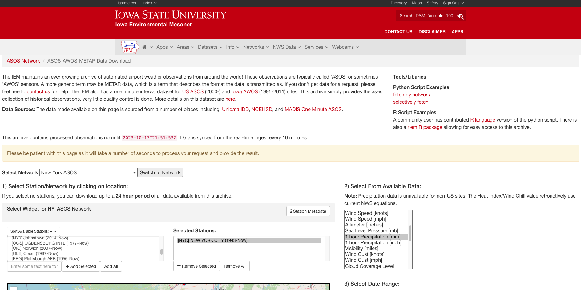
Screenshot of ASOS Data Download.
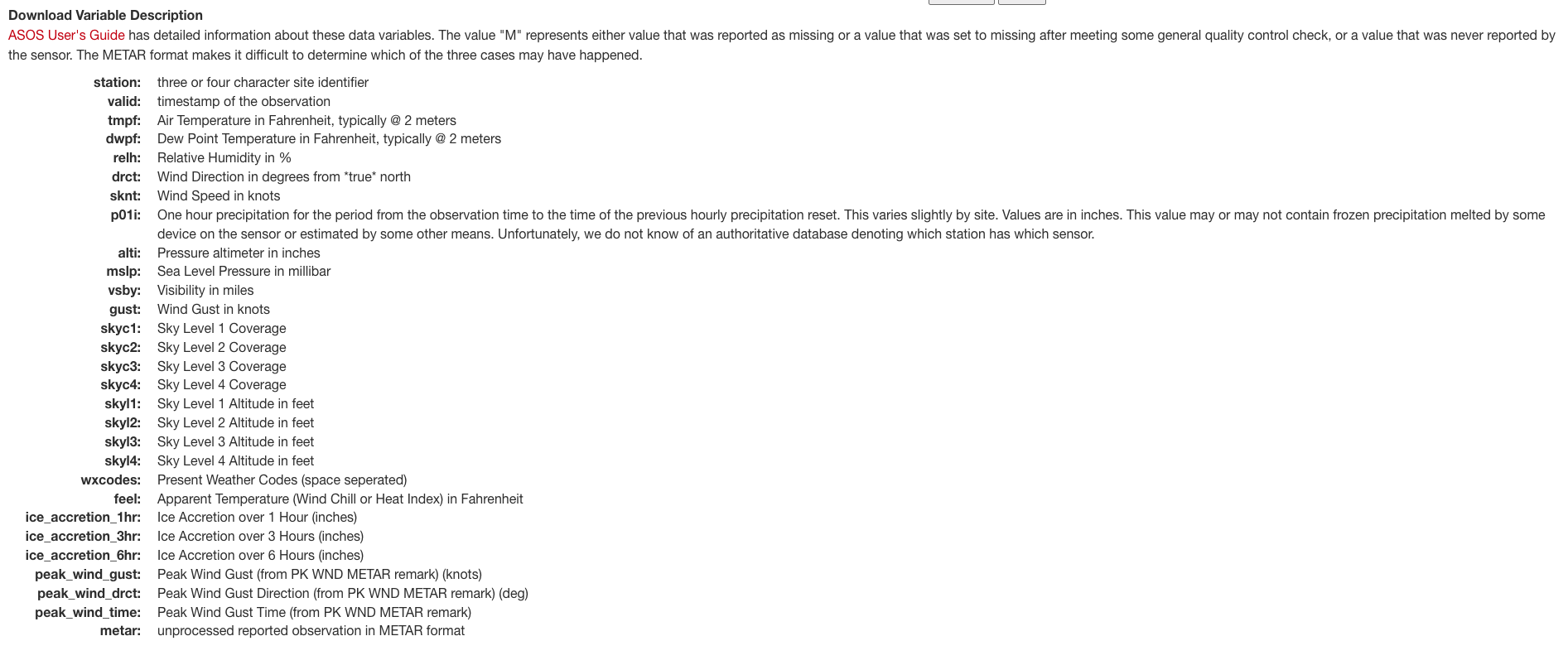
Screenshot of ASOS Data Dictionary.
path = 'data/hourly-precipitation.csv'

df = pd.read_csv(path)
print('shape of data: {}'.format(df.shape))
df['datetime'] = pd.to_datetime(df['datetime'])

# preview data
df.head()
shape of data: (303920, 7)
| station | valid | datetime | lon | lat | p01mm | p01in | |
|---|---|---|---|---|---|---|---|
| 0 | NYC | 1965-01-02 18:00 | 1965-01-02 18:00:00 | -73.9693 | 40.779 | 0.51 | 0.0201 |
| 1 | NYC | 1965-01-02 21:00 | 1965-01-02 21:00:00 | -73.9693 | 40.779 | 1.27 | 0.0500 |
| 2 | NYC | 1965-01-03 00:00 | 1965-01-03 00:00:00 | -73.9693 | 40.779 | 1.27 | 0.0500 |
| 3 | NYC | 1965-01-03 03:00 | 1965-01-03 03:00:00 | -73.9693 | 40.779 | NaN | NaN |
| 4 | NYC | 1965-01-03 06:00 | 1965-01-03 06:00:00 | -73.9693 | 40.779 | NaN | NaN |
# review column nulls and dtypes
df.info()
<class 'pandas.core.frame.DataFrame'>
RangeIndex: 303920 entries, 0 to 303919
Data columns (total 7 columns):
 #   Column    Non-Null Count   Dtype
---  ------    --------------   -----
 0   station   303920 non-null  object
 1   valid     303920 non-null  object
 2   datetime  303920 non-null  datetime64[ns]
 3   lon       303920 non-null  float64
 4   lat       303920 non-null  float64
 5   p01mm     112502 non-null  float64
 6   p01in     112502 non-null  float64
dtypes: datetime64[ns](1), float64(4), object(2)
memory usage: 16.2+ MB
print('datetime bounds of analysis:\n')
print('date min: {}'.format(df['datetime'].min()))
print('date max: {}'.format(df['datetime'].max()))
datetime bounds of analysis:

date min: 1965-01-02 18:00:00
date max: 2023-10-08 23:51:00
Analysis of Extreme Rainfall
The standard design criterion in New York City is to use the intensity-duration values based on a storm with a 5-year return period (e.g., 1.75 inches per hour for a one hour storm; 20 percent chance of occurrence in any given year) to calculate how large the sewer pipes need to be sized to appropriately manage stormwater. Certain older areas of the City are designed to a 3-year storm event. The sewer design flow is then determined by application of an equation using a runoff coefficient, a rainfall intensity determined from an equation derived from the IDF analysis, and the contributory drainage area. The design of combined sewers includes allowance for the sanitary flows. The IDF curve currently used by New York City is based on historical data from 1903-1951. With climate change, the intensity and duration of a storm with a 5-year return period is likely to increase, and therefore the current curve may not be adequate for designing infrastructure that is to last decades.
Source: https://www.nyc.gov/assets/orr/pdf/publications/stormwater-resiliency-plan.pdf
counts = (
    df
    .loc[df['p01in'] >= 1.75]
    .shape[0]
)

print('Number of hourly observations with >= 1.75 inches of precipitation: {}'.format(counts))
Number of hourly observations with >= 1.75 inches of precipitation: 4
# records in print view
records = (
    df
    .loc[df['p01in'] >= 1.75, ['valid', 'p01in']]
    .rename(columns={'valid':'date', 'p01in':'inches'})
    .sort_values(by='inches', ascending=False)
    .set_index([pd.Series(range(1, counts + 1))])
)

records
| date | inches | |
|---|---|---|
| 1 | 2021-09-02 01:51 | 3.1500 |
| 2 | 2023-09-29 13:51 | 1.9598 |
| 3 | 2021-08-22 03:51 | 1.9402 |
| 4 | 2004-09-08 11:51 | 1.7598 |
Table xx: Top precipitation events of over 1.75 inches of rainfall per hour at Central Park, NYC.
# top 20 hourly precipitation events
records = (
    df
    .loc[:, ['valid', 'p01in']]
    .rename(columns={'valid':'date', 'p01in':'inches'})
    .sort_values(by='inches', ascending=False)
    .head(20)
    .set_index([pd.Series(range(1, 20 + 1))])
)

records
| date | inches | |
|---|---|---|
| 1 | 2021-09-02 01:51 | 3.1500 |
| 2 | 2023-09-29 13:51 | 1.9598 |
| 3 | 2021-08-22 03:51 | 1.9402 |
| 4 | 2004-09-08 11:51 | 1.7598 |
| 5 | 2005-08-14 23:51 | 1.7000 |
| 6 | 2007-08-08 10:51 | 1.7000 |
| 7 | 2018-08-11 12:51 | 1.6598 |
| 8 | 2020-08-12 20:51 | 1.6299 |
| 9 | 1967-07-03 09:00 | 1.5799 |
| 10 | 2006-08-10 23:51 | 1.5701 |
| 11 | 2021-07-08 21:51 | 1.5598 |
| 12 | 1973-08-02 15:00 | 1.5098 |
| 13 | 2021-09-02 02:51 | 1.5000 |
| 14 | 2010-10-01 09:51 | 1.4799 |
| 15 | 2009-01-17 16:51 | 1.4299 |
| 16 | 2009-01-17 23:51 | 1.4098 |
| 17 | 2021-08-22 02:51 | 1.3799 |
| 18 | 2021-07-12 06:51 | 1.3500 |
| 19 | 2022-12-23 09:51 | 1.3299 |
| 20 | 2009-01-17 21:51 | 1.3299 |
Table xx: Top 20 precipitation events per hour at Central Park, NYC.
fig, ax = plt.subplots(figsize=(8, 6))

sns.lineplot(
    x=df['datetime'],
    y=df['p01in'],
    label='Precipitation'
)

plt.title(
    'Hourly Precipitation in Central Park, NYC',
    fontsize=12,
    pad=10
)

plt.axhline(y=1.75, color='r',linestyle='--', label='1.75 inches')

plt.legend(loc=2)
plt.xlabel('Hourly Observations', fontsize=12)
plt.ylabel('Precipitation (inches)', fontsize=12)
plt.tight_layout()
Figure xx: Hourly Precipitation in Central Park, NYC. The figure above looks a bit weird with big chunks of missing data. This is only to demonstrate the distribution of values and extreme values. There is a big gap in the hourly data from 1985 to 2000.
Daily Precipitation Data
I used NOAA's NCEI Climate Data Online Daily Summaries.
NCEI Climate Data Online's Daily Summaries, NY CITY CENTRAL PARK, NY US
Source: https://www.ncei.noaa.gov/cdo-web/datasets/GHCND/stations/GHCND:USW00094728/detail
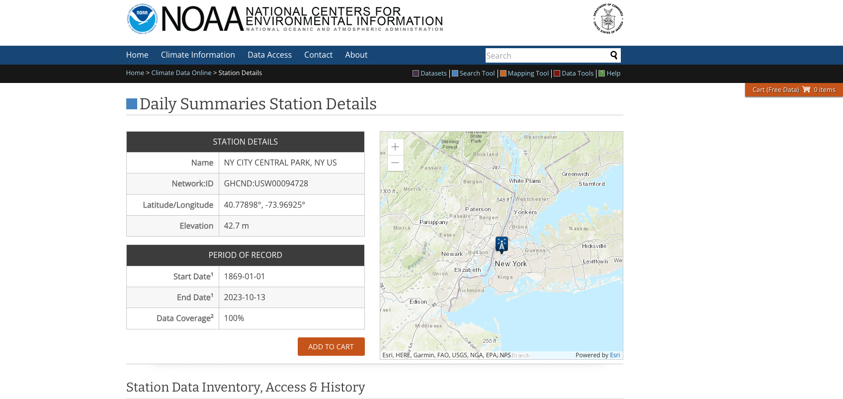
Screenshot of NCEI Climate Data Online's Daily Summaries.
# download of data was performed manually by me from NCEI above
df = pd.read_csv('data/daily-precipitation.csv')

## to datetime
df['datetime'] = pd.to_datetime(df['DATE'])

# preview data
print('shape of data: {}'.format(df.shape))
df.head()
shape of data: (56535, 9)
| STATION | NAME | LATITUDE | LONGITUDE | ELEVATION | DATE | PRCP | PRCP_ATTRIBUTES | datetime | |
|---|---|---|---|---|---|---|---|---|---|
| 0 | USW00094728 | NY CITY CENTRAL PARK, NY US | 40.77898 | -73.96925 | 42.7 | 1869-01-01 | 0.75 | ,,Z, | 1869-01-01 |
| 1 | USW00094728 | NY CITY CENTRAL PARK, NY US | 40.77898 | -73.96925 | 42.7 | 1869-01-02 | 0.03 | ,,Z,null | 1869-01-02 |
| 2 | USW00094728 | NY CITY CENTRAL PARK, NY US | 40.77898 | -73.96925 | 42.7 | 1869-01-03 | 0.00 | T,,Z,null | 1869-01-03 |
| 3 | USW00094728 | NY CITY CENTRAL PARK, NY US | 40.77898 | -73.96925 | 42.7 | 1869-01-04 | 0.18 | ,,Z,null | 1869-01-04 |
| 4 | USW00094728 | NY CITY CENTRAL PARK, NY US | 40.77898 | -73.96925 | 42.7 | 1869-01-05 | 0.05 | ,,Z,null | 1869-01-05 |
print('datetime bounds of analysis:\n')
print('date min: {}'.format(df['datetime'].min()))
print('date max: {}'.format(df['datetime'].max()))
datetime bounds of analysis:

date min: 1869-01-01 00:00:00
date max: 2023-10-15 00:00:00
The Number of Days with Extreme Rainfall
Recent academic studies show that sub-daily rainfall intensity may increase over the coming decades.5 Since rainfall information started being collected, the number of days with extreme rainfall (defined as days of rainfall over 1.75 inches in Central Park) has increased.6
Source: https://www.nyc.gov/assets/orr/pdf/publications/stormwater-resiliency-plan.pdf
counts = (
    df.loc[df['PRCP'] >= 1.75]
    .shape[0]
)

print('Total number of daily observations with >= 1.75 inches of precipitation: {}'.format(counts))
Total number of daily observations with >= 1.75 inches of precipitation: 545
# top 20 daily precipitation events
records = (
    df
    .loc[:, ['datetime', 'PRCP']]
    .rename(columns={'datetime':'date', 'PRCP':'inches'})
    .sort_values(by='inches', ascending=False)
    .head(20)
    .set_index([pd.Series(range(1, 20 + 1))])
)

records
| date | inches | |
|---|---|---|
| 1 | 1882-09-23 | 8.28 |
| 2 | 2007-04-15 | 7.57 |
| 3 | 1977-11-08 | 7.40 |
| 4 | 1903-10-09 | 7.33 |
| 5 | 2021-09-01 | 7.13 |
| 6 | 2011-08-14 | 5.81 |
| 7 | 1972-11-08 | 5.60 |
| 8 | 1966-09-21 | 5.54 |
| 9 | 2023-09-29 | 5.48 |
| 10 | 1999-09-16 | 5.02 |
| 11 | 1913-10-01 | 4.98 |
| 12 | 2014-04-30 | 4.97 |
| 13 | 1934-09-08 | 4.86 |
| 14 | 1909-08-16 | 4.80 |
| 15 | 1873-08-20 | 4.80 |
| 16 | 1990-08-10 | 4.64 |
| 17 | 2021-08-21 | 4.45 |
| 18 | 1996-10-19 | 4.35 |
| 19 | 1983-04-10 | 4.31 |
| 20 | 1903-10-08 | 4.30 |
Table xx: Top 20 precipitation events per day at Central Park, NYC.
fig, ax = plt.subplots(figsize=(8, 6))

sns.lineplot(
    x=df.set_index('datetime').index,
    y=df['PRCP'],
    label='Precipitation'
)

plt.title(
    'Daily Precipitation in Central Park, NYC',
    fontsize=12,
    pad=10
)

plt.axhline(y=1.75, color='r', linestyle='--', label='1.75 inches')

plt.legend(loc='upper center')
plt.xlabel('Daily', fontsize=12)
plt.ylabel('Precipitation (inches)', fontsize=12)
plt.tight_layout()
Figure xx: Daily precipitation in Central Park, NYC.
# assign flag to extreme days
df.loc[df['PRCP'] >= 1.75, ['threshold']] = 1

# count days and bin data by decade
bins = [x for x in range(1860, 2040, 10)]
df['bins'] = pd.cut(df['datetime'].dt.year, bins=bins)

data = (
    df
    .groupby(by='bins')['threshold']
    .sum()
    .astype(int)
    .rename('count')
    .reset_index()
)

# clipping incomplete decades, remove from plot
data = data.iloc[1:-1, :].reset_index(drop=True)
data
| bins | count | |
|---|---|---|
| 0 | (1870, 1880] | 33 |
| 1 | (1880, 1890] | 30 |
| 2 | (1890, 1900] | 26 |
| 3 | (1900, 1910] | 41 |
| 4 | (1910, 1920] | 36 |
| 5 | (1920, 1930] | 27 |
| 6 | (1930, 1940] | 32 |
| 7 | (1940, 1950] | 21 |
| 8 | (1950, 1960] | 22 |
| 9 | (1960, 1970] | 25 |
| 10 | (1970, 1980] | 55 |
| 11 | (1980, 1990] | 50 |
| 12 | (1990, 2000] | 41 |
| 13 | (2000, 2010] | 46 |
| 14 | (2010, 2020] | 42 |
fig, ax = plt.subplots(figsize=(8, 6))

data.plot.bar(
    x='bins',
    y='count',
    rot=45,
    legend=None,
    ax=ax
)

plt.title('Count of Days Greater Than or Equal to 1.75 Inches of Rainfall per Decade', fontsize=12)
plt.xlabel('Decade', fontsize=12)
plt.ylabel('Count of Days', fontsize=12)
plt.tight_layout()
plt.savefig('figures/precip-cover-photo.png', dpi=250, bbox_inches='tight')
Figure xx: Count of days greater than or equal to 1.75 inches of rainfall per decade.
NOAA ATLAS 14 Point Precipitation Frequency Estimates
NOAA Atlas 14 estimates are used to design, plan, and manage much of the Nation's infrastructure for a wide variety of purposes under federal, state, and local regulations. NOAA Atlas 14 estimates replace estimates previously published by NOAA in the early 1960s and '70s and cover a range of storm durations from 5-minutes through 60-days, for average recurrence intervals of 1-year through 1,000-year. Compared to previous volumes, Atlas 14 estimates benefit from use of better-quality data (e.g. precipitation stations with longer period of record, increased station density, etc.), enhanced quality control methods, consideration of uncertainties, and improved frequency analysis and spatial interpolation methods that account for variation in terrain, proximity to the coastline etc.
Source: https://www.weather.gov/owp/hdsc
Atlas 14 is so influencial with the country's design standards, I figured I would add a section about it. The first set of screen shots are from NOAA's Atlas 14, and the last one is the flood scenarios from the NYC Stormwater Flood Maps. It's good to understand and communicate the relationship between duration (e.g. 60-min), average reoccurance interval (e.g. 100-year), precipitation levels and potential flood depths.
Station Name: NY CITY CNTRL PARK
Below are screenshots and data for Central Park, NYC.
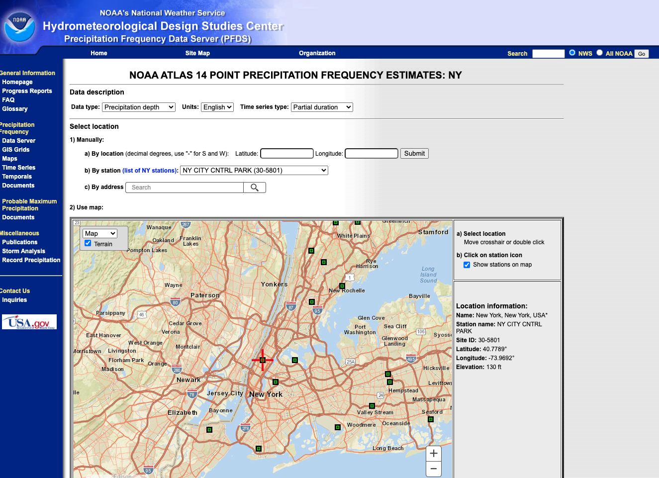
Screenshot of the landing page.
Source: https://hdsc.nws.noaa.gov/pfds/pfds_map_cont.html?bkmrk=ny
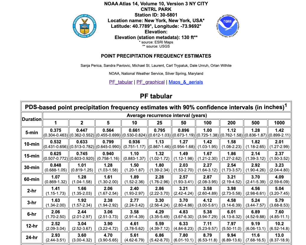
Table caption from NOAA:
Precipitation frequency (PF) estimates in this table are based on frequency analysis of partial duration series (PDS). Numbers in parenthesis are PF estimates at lower and upper bounds of the 90% confidence interval. The probability that precipitation frequency estimates (for a given duration and average recurrence interval) will be greater than the upper bound (or less than the lower bound) is 5%. Estimates at upper bounds are not checked against probable maximum precipitation (PMP) estimates and may be higher than currently valid PMP values. Please refer to NOAA Atlas 14 document for more information.
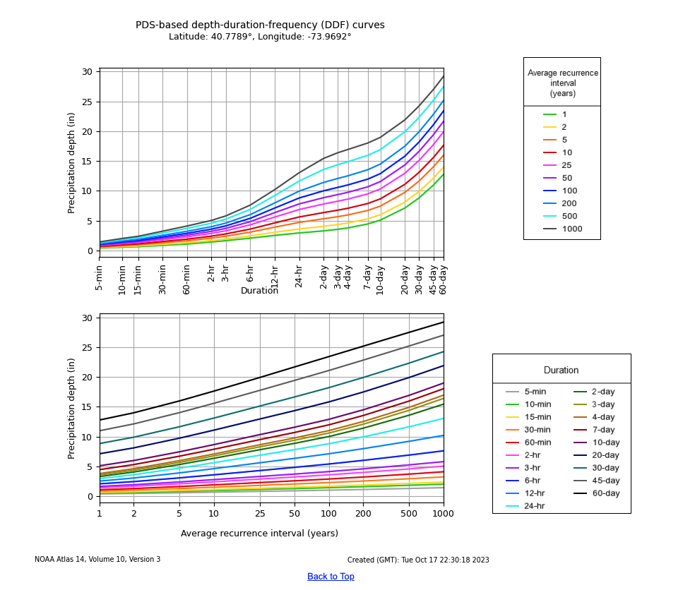
The flood scenarios for the NYC Stormwater Flood Maps are below. Things to note: extreme scenario consists of Deep and Continous Flooding depths of 1 ft. and greater, and Sea Level Rise heights of + 4.8 ft.

Source: https://experience.arcgis.com/experience/6f4cc60710dc433585790cd2b4b5dd0e