Accessing 3DEP Lidar COG data with the Planetary Computer STAC API¶

The Planetary Computer includes a group of datasets derived from the USGS 3DEP Lidar program. The raw data are available as a collection of COPC assets. In addition, various derived products like Intensity and Height Above Ground are available.

This notebook demonstrates working with the derived COG products. For more on working with the COPC data, see its example notebook.

Environment setup¶

This notebook works with or without an API key, but you will be given more permissive access to the data with an API key. The Planetary Computer Hub is pre-configured to use your API key.

In [1]:

import pystac_client
import planetary_computer
import rasterio
import numpy as np
import matplotlib
import matplotlib.pyplot as plt


# Set the environment variable PC_SDK_SUBSCRIPTION_KEY, or set it here.
# The Hub sets PC_SDK_SUBSCRIPTION_KEY automatically.
# pc.settings.set_subscription_key(<YOUR API Key>)

client = pystac_client.Client.open(
    "https://planetarycomputer.microsoft.com/api/stac/v1/",
    modifier=planetary_computer.sign_inplace,
)

We'll use the STAC API to search for items from these various collections over Washington D.C.

In [2]:

collections = [
    "3dep-lidar-hag",
    "3dep-lidar-dsm",
    "3dep-lidar-pointsourceid",
    "3dep-lidar-intensity",
    "3dep-lidar-dtm",
    "3dep-lidar-dtm-native",
    "3dep-lidar-returns",
    "3dep-lidar-classification",
]

search = client.search(
    collections=collections,
    intersects={
        "type": "Point",
        "coordinates": [-77.10058811018344, 38.838335717896314],
    },
    datetime="2018",
)
items = {x.collection_id: x for x in search.get_all_items()}
items

Out[2]:

{'3dep-lidar-returns': <Item id=USGS_LPC_VA_Fairfax_County_2018-returns-5m-2-1>,
 '3dep-lidar-pointsourceid': <Item id=USGS_LPC_VA_Fairfax_County_2018-pointsourceid-5m-2-1>,
 '3dep-lidar-intensity': <Item id=USGS_LPC_VA_Fairfax_County_2018-intensity-2m-5-3>,
 '3dep-lidar-hag': <Item id=USGS_LPC_VA_Fairfax_County_2018-hag-2m-5-3>,
 '3dep-lidar-dtm-native': <Item id=USGS_LPC_VA_Fairfax_County_2018-dtm_native-2m-5-3>,
 '3dep-lidar-dtm': <Item id=USGS_LPC_VA_Fairfax_County_2018-dtm-2m-5-3>,
 '3dep-lidar-dsm': <Item id=USGS_LPC_VA_Fairfax_County_2018-dsm-2m-5-3>,
 '3dep-lidar-classification': <Item id=USGS_LPC_VA_Fairfax_County_2018-classification-2m-5-3>}

In [3]:

items["3dep-lidar-returns"].assets["data"].href

Out[3]:

'https://usgslidareuwest.blob.core.windows.net/usgs-3dep-cogs/usgs-cogs/USGS_LPC_VA_Fairfax_County_2018/numberofreturns/USGS_LPC_VA_Fairfax_County_2018-returns-5m-2-1.tif?st=2022-08-08T14%3A32%3A43Z&se=2022-08-16T14%3A32%3A43Z&sp=rl&sv=2021-06-08&sr=c&skoid=c85c15d6-d1ae-42d4-af60-e2ca0f81359b&sktid=72f988bf-86f1-41af-91ab-2d7cd011db47&skt=2022-08-09T14%3A32%3A42Z&ske=2022-08-16T14%3A32%3A42Z&sks=b&skv=2021-06-08&sig=pNxIEF9eBA0rbTbQIV5i/XqtwzBzzqMHOw7J7JWR3TA%3D'

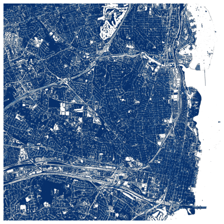
Height Above Ground¶

This COG type is generated using the Z dimension of the COPC data data and removes noise, water, and using pdal.filters.smrf followed by pdal.filters.hag_nn.

In [4]:

ds = rasterio.open(items["3dep-lidar-hag"].assets["data"].href).read().squeeze()

This COG has a special colormap we can use to visualize its values correctly.

In [5]:

pairs = [
    ((-900, 1), (0, 0, 0, 0)),
    ((1, 2), (205, 224, 241, 255)),
    ((2, 3), (175, 209, 231, 255)),
    ((3, 4), (137, 190, 220, 255)),
    ((4, 5), (96, 166, 210, 255)),
    ((5, 6), (34, 114, 181, 255)),
    ((6, 7), (10, 84, 158, 255)),
    ((7, 100), (8, 48, 107, 255)),
]


intervals, colors = zip(*pairs)
nodes = np.array([x[1] for x in intervals]).astype(float)
nodes -= np.abs(nodes.min())
nodes /= nodes.max()


colors = [np.asarray(c) / 255 for c in colors]

cmap = matplotlib.colors.LinearSegmentedColormap.from_list(
    "hag", list(zip(nodes, colors))
)

In [6]:

fig, ax = plt.subplots(figsize=(8, 8))

ax.imshow(cmap(ds), cmap=cmap)
ax.set_axis_off()

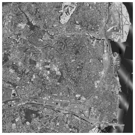
Intensity¶

This collection is derived from the USGS 3DEP COPC collection. It is a collection of Cloud Optimized GeoTIFFs representing the pulse return magnitude.

In [7]:

ds = rasterio.open(items["3dep-lidar-intensity"].assets["data"].href).read().squeeze()

fig, ax = plt.subplots(figsize=(8, 8))

ax.imshow(ds, cmap="gray")
ax.set_axis_off()

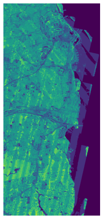
Returns¶

This collection is derived from the USGS 3DEP COPC collection. It is a collection of Cloud Optimized GeoTIFFs representing the number of returns for a given pulse.

In [8]:

ds = rasterio.open(items["3dep-lidar-returns"].assets["data"].href).read().squeeze()
np.putmask(ds, ds < 1, 0)
np.putmask(ds, ds >= 7, 7)

fig, ax = plt.subplots(figsize=(8, 8))

ax.imshow(ds)
ax.set_axis_off()

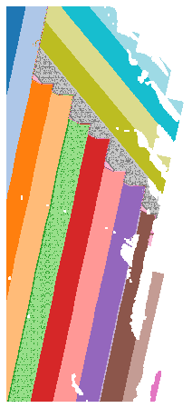
Classification¶

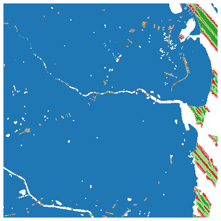
This collection is derived from the USGS 3DEP COPC collection. It uses the ASPRS (American Society for Photogrammetry and Remote Sensing) Lidar point classification. See LAS specification for details.

In [9]:

ds = (
    rasterio.open(items["3dep-lidar-classification"].assets["data"].href)
    .read()
    .squeeze()
)
ds = np.where(ds > 0, ds, np.nan)
fig, ax = plt.subplots(figsize=(8, 8))

ax.imshow(ds, cmap="tab20")
ax.set_axis_off()

DSM¶

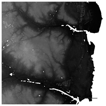
This collection is derived from the USGS 3DEP COPC collection. It creates a Digital Surface Model (DSM) using pdal.filters.range to output a collection of Cloud Optimized GeoTIFFs, removing all points that have been classified as noise.

In [10]:

ds = rasterio.open(items["3dep-lidar-dsm"].assets["data"].href).read().squeeze()
ds = np.where(ds > 0, ds, np.nan)
fig, ax = plt.subplots(figsize=(8, 8))

ax.imshow(ds, cmap="gray")
ax.set_axis_off()

DTM¶

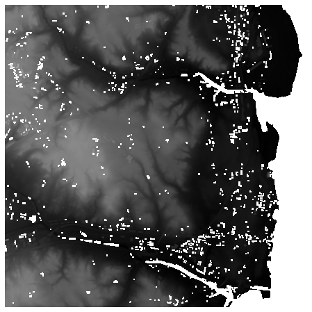
This collection is derived from the USGS 3DEP COPC collection. It creates a Digital Terrain Model (DTM) using pdal.filters.smrf to output a collection of Cloud Optimized GeoTIFFs.

In [11]:

ds = rasterio.open(items["3dep-lidar-dtm"].assets["data"].href).read().squeeze()
ds = np.where(ds > 0, ds, np.nan)
fig, ax = plt.subplots(figsize=(8, 8))

ax.imshow(ds, cmap="gray")
ax.set_axis_off()

DTM Native¶

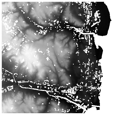
This collection is derived from the USGS 3DEP COPC collection. It creates a Digital Terrain Model (DTM) using the vendor provided (native) ground classification and pdal.filters.range to output a collection of Cloud Optimized GeoTIFFs, removing all points that have been classified as noise.

In [12]:

ds = rasterio.open(items["3dep-lidar-dtm-native"].assets["data"].href).read().squeeze()
ds = np.where(ds > 0, ds, np.nan)
fig, ax = plt.subplots(figsize=(8, 8))

ax.imshow(ds, cmap="gray")
ax.set_axis_off()

Point Source ID¶

This collection is derived from the USGS 3DEP COPC collection. It is a collection of Cloud Optimized GeoTIFFs representing the file source ID from which the point originated. Zero indicates that the point originated in the current file.

In [13]:

ds = (
    rasterio.open(items["3dep-lidar-pointsourceid"].assets["data"].href)
    .read()
    .squeeze()
)
ds = np.where(ds > 0, ds, np.nan)
fig, ax = plt.subplots(figsize=(8, 8))

ax.imshow(ds, cmap="tab20")
ax.set_axis_off()