Accessing Forest Inventory and Analysis data with the Planetary Computer STAC API¶

This notebook demonstrates accessing Forest Inventory and Analysis (FIA) data from the Planetary Computer STAC API.

The Forest Inventory and Analysis collection contains many tables, and each STAC table corresponds to one STAC item in the FIA collection. In this example, we'll use a few of the tables to estimate the total amount of aboveground carbon, in pounds, per US county.

This example builds on the plot estimation example from the rfia package.

In [1]:

from cartopy import crs as ccrs
import dask_gateway
import dask_geopandas
import dask.dataframe as dd
import geopandas
import matplotlib.pyplot as plt
import numpy as np
import pandas as pd
import pystac_client
import planetary_computer

The tree table below is relatively large, so we'll process it in parallel on a Dask cluster. The example will still run without a cluster, it will just take longer.

In [2]:

cluster = dask_gateway.GatewayCluster()
cluster.scale(16)
client = cluster.get_client()
cluster

VBox(children=(HTML(value='<h2>GatewayCluster</h2>'), HBox(children=(HTML(value='\n<div>\n<style scoped>\n    …

Data Access¶

We'll use two datsaets

tree: Information on each tree 1″ in diameter or larger, linked to plot and cond.
plot: Information relevant to each 1-acre field plot where the samples were collected.

All of these are available in Azure Blob Storage as parquet datasets that can be read, for example, by dask.dataframe.

In [3]:

catalog = pystac_client.Client.open(
    "https://planetarycomputer.microsoft.com/api/stac/v1",
    modifier=planetary_computer.sign_inplace,
)
fia = catalog.get_collection("fia")
fia

Out[3]:

<CollectionClient id=fia>

In [4]:

plot_item = fia.get_item("plot")
tree_item = fia.get_item("tree")

And now we can read the items using dask.dataframe. We make sure to pass the storage_options included in the data asset.

In [5]:

plot = dd.read_parquet(
    plot_item.assets["data"].href,
    columns=["CN", "STATECD", "COUNTYCD"],
    storage_options=plot_item.assets["data"].extra_fields["table:storage_options"],
    engine="pyarrow",
)
tree = dd.read_parquet(
    tree_item.assets["data"].href,
    columns=["PLT_CN", "CONDID", "TREE", "DRYBIO_AG", "CARBON_AG", "TPA_UNADJ"],
    storage_options=tree_item.assets["data"].extra_fields["table:storage_options"],
    engine="pyarrow",
    filters=[("CONDID", "==", 1)],
)

Join the datasets¶

The three datasets can be joined on their various keys. Since tree is relatively large, we'll join the other (smaller, in-memory) dataframes to it.

In [6]:

df = tree.merge(plot.assign(PLT_CN=plot.CN).compute(), on="PLT_CN").assign(
    bio=lambda df: df.DRYBIO_AG * df.TPA_UNADJ / 2000,
    carbon=lambda df: df.CARBON_AG * df.TPA_UNADJ / 2000,
)
df

Out[6]:

Dask DataFrame Structure:

	PLT_CN	CONDID	TREE	DRYBIO_AG	CARBON_AG	TPA_UNADJ	CN	STATECD	COUNTYCD	bio	carbon
npartitions=160
	int64	int64	int64	float64	float64	float64	int64	int64	int64	float64	float64
	...	...	...	...	...	...	...	...	...	...	...
...	...	...	...	...	...	...	...	...	...	...	...
	...	...	...	...	...	...	...	...	...	...	...
	...	...	...	...	...	...	...	...	...	...	...

Dask Name: assign, 1921 tasks

Compute per-county summaries¶

The df dataframe now includes the state and county FIPS codes, and the (adjusted) aboveground carbon and biomass. We'll group by the geographic boundaries and sum the aboveground carbon and biomass.

In [7]:

%%time
result = (
    df.groupby(["STATECD", "COUNTYCD"])[["bio", "carbon"]]
    .sum()
    .compute()
    .reset_index()
    .assign(
        STATE=lambda df: df["STATECD"].astype("string").str.pad(2, fillchar="0"),
        COUNTY=lambda df: df["COUNTYCD"].astype("string").str.pad(3, fillchar="0"),
    )
    .drop(columns=["STATECD", "COUNTYCD"])
)
result.head()

CPU times: user 259 ms, sys: 36.5 ms, total: 296 ms
Wall time: 35.2 s

Out[7]:

	bio	carbon	STATE	COUNTY
0	9130.179946	4565.090000	01	001
1	27163.826785	13565.771340	01	003
2	15567.843806	7774.593220	01	005
3	16643.533828	8321.766954	01	007
4	8742.498366	4364.876867	01	009

Plot the results¶

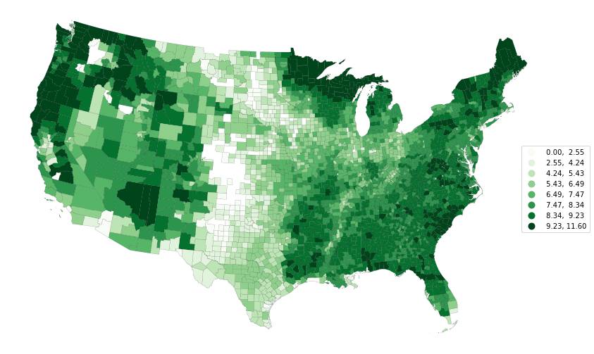
Now we'll make a chloropleth for the results. We just need to join in the actual geographic boundaries of the datasets, which we can get with geopandas.

In [8]:

census_item = catalog.get_collection("us-census").get_item(
    "2020-cb_2020_us_county_500k"
)

counties = (
    dask_geopandas.read_parquet(
        census_item.assets["data"].href,
        storage_options=census_item.assets["data"].extra_fields[
            "table:storage_options"
        ],
        columns=["STATEFP", "COUNTYFP", "geometry"],
    ).rename(columns={"STATEFP": "STATE", "COUNTYFP": "COUNTY"})
).compute()

Finally, we'll slice the data down to the continental United States (the dataset covers Hawaii, Alaska, and several territories).

In [9]:

gdf = geopandas.GeoDataFrame(pd.merge(result, counties, on=["STATE", "COUNTY"]))
df_conus = gdf.cx[-124.784:-66.951, 24.744:49.346]
df_conus.head()

Out[9]:

	bio	carbon	STATE	COUNTY	geometry
0	9130.179946	4565.090000	01	001	POLYGON ((-86.92120 32.65754, -86.92035 32.658...
1	27163.826785	13565.771340	01	003	POLYGON ((-88.02858 30.22676, -88.02399 30.230...
2	15567.843806	7774.593220	01	005	POLYGON ((-85.74803 31.61918, -85.74544 31.618...
3	16643.533828	8321.766954	01	007	POLYGON ((-87.42194 33.00338, -87.31854 33.006...
4	8742.498366	4364.876867	01	009	POLYGON ((-86.96336 33.85822, -86.95967 33.857...

Finally, we'll plot the (log) of the estimated carbon stored above ground by the trees.

In [10]:

crs = ccrs.LambertConformal()
fig, ax = plt.subplots(subplot_kw={"projection": crs}, figsize=(16, 9))
df_conus.assign(carbon=np.log(df_conus.carbon + 1)).to_crs(crs.proj4_init).plot(
    column="carbon",
    cmap="Greens",
    edgecolor="k",
    scheme="natural_breaks",
    k=8,
    ax=ax,
    linewidths=0.1,
    legend=True,
)

# Shift the legend
bbox = ax.legend_.get_bbox_to_anchor().transformed(ax.transAxes.inverted())
bbox.x0 += 0.075
bbox.x1 += 0.075
bbox.y0 -= 0.4
bbox.y1 -= 0.4
ax.legend_.set_bbox_to_anchor(bbox)

ax.axis("off");

Next Steps¶

Now that you've an introduction to the Forest Inventory and Analysis dataset, learn more with

The Reading tabular data quickstart for an introduction to tabular data on the Planeatry Computer