Accessing Harmonized Global Biomass data with the Planetary Computer STAC API¶

The Harmonized Global Biomass (HGB) dataset provides temporally consistent and harmonized global maps of aboveground and belowground biomass carbon density for the year 2010 at 300m resolution.

This notebook provides an example of accessing HGB data using the Planetary Computer STAC API, inspecting the data assets in the catalog, and doing some simple processing and plotting of the data from the Cloud Optimized GeoTIFF source.

Environment setup¶

This notebook works with or without an API key, but you will be given more permissive access to the data with an API key. The Planetary Computer Hub is pre-configured to use your API key.

In [1]:

import matplotlib.pyplot as plt
import pystac_client
import planetary_computer
import rioxarray
import dask.distributed

Data access¶

The datasets hosted by the Planetary Computer are available from Azure Blob Storage. We'll use pystac-client to search the Planetary Computer's STAC API for the subset of the data that we care about, and then we'll load the data directly from Azure Blob Storage. We'll specify a modifier so that we can access the data stored in the Planetary Computer's private Blob Storage Containers. See Reading from the STAC API and Using tokens for data access for more.

In [2]:

catalog = pystac_client.Client.open(
    "https://planetarycomputer.microsoft.com/api/stac/v1",
    modifier=planetary_computer.sign_inplace,
)

items = list(catalog.get_collection("hgb").get_all_items())
print(f"Returned {len(items)} Items")

Returned 1 Items

You'll see we only returned a single item for the entire collection. This is a bit different from other types of datasets on the Planetary Computer. Each of the assets are represented by a single global raster at a single temporal resolution.

Let's see what assets are associated with this item:

In [3]:

item = items[0]
print(*[f"{key}: {asset.title}" for key, asset in item.assets.items()], sep="\n")

aboveground: Global above-ground biomass
belowground: Global below-ground biomass
aboveground_uncertainty: Uncertainty associated with global above-ground biomass
belowground_uncertainty: Uncertainty associated with global below-ground biomass
tilejson: TileJSON with default rendering
rendered_preview: Rendered preview

Load the variable of interest¶

In [4]:

da = rioxarray.open_rasterio(
    item.assets["aboveground"].href, chunks=dict(x=2560, y=2560)
)

# Transform our data array to a dataset by selecting the only data variable ('band')
# renaming it to something useful ('biomass')
ds = da.to_dataset(dim="band").rename({1: "biomass"})
ds

Out[4]:

<xarray.Dataset>
Dimensions:      (y: 52201, x: 129600)
Coordinates:
  * x            (x) float64 -180.0 -180.0 -180.0 -180.0 ... 180.0 180.0 180.0
  * y            (y) float64 84.0 84.0 83.99 83.99 ... -60.99 -61.0 -61.0 -61.0
    spatial_ref  int64 0
Data variables:
    biomass      (y, x) uint16 dask.array<chunksize=(2560, 2560), meta=np.ndarray>
Attributes:
    AREA_OR_POINT:       Area
    DataType:            Generic
    OVR_RESAMPLING_ALG:  NEAREST
    scale_factor:        1.0
    add_offset:          0.0

Plot global aboveground biomass¶

We'll be loading in a global 300m raster, so let's spin up a distributed Dask cluster to parallelize our reads and computation. You can use the dashboard link to monitor resources and progress on the cluster.

In [5]:

dask_client = dask.distributed.Client()
print(dask_client.dashboard_link)

/user/taugspurger@microsoft.com/proxy/8787/status

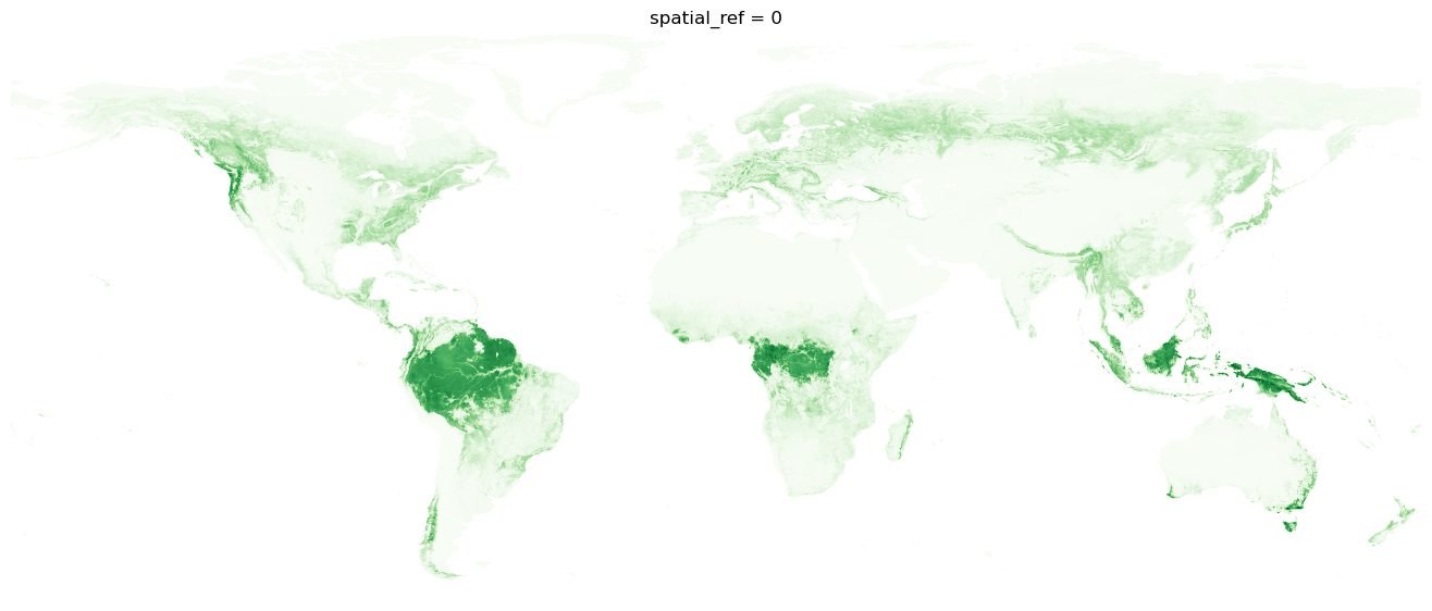
For this global plot, it's ok to lose some detail in our rendering. First we'll downsample the entire dataset by a factor of 100 on each spatial dimension and drop drop any values at zero or below.

In [6]:

%%time
factor = 100
coarse_biomass = (
    ds.biomass.coarsen(dim={"x": factor, "y": factor}, boundary="trim").mean().compute()
)

# Filter out nodata
coarse_biomass = coarse_biomass.where(coarse_biomass > 0)
coarse_biomass.shape

CPU times: user 16.7 s, sys: 1.49 s, total: 18.2 s
Wall time: 42.6 s

Out[6]:

(522, 1296)

With our dataset nicely reduced, we can plot the above ground biomass for the planet.

In [7]:

h, w = coarse_biomass.shape
dpi = 100
fig = plt.figure(frameon=False, figsize=(w / dpi, h / dpi), dpi=dpi)
ax = plt.Axes(fig, [0.0, 0.0, 1.0, 1.0])
ax.set_axis_off()
fig.add_axes(ax)
coarse_biomass.plot(cmap="Greens", add_colorbar=False)
plt.show();