Accessing MODIS imagery data with the Planetary Computer STAC API¶

The planetary computer hosts three imagery-related MODIS 6.1 products:

Surface Reflectance 8-Day 500m (09A1)
Surface Reflectance 8-Day 250m (09Q1)
Nadir BRDF-Adjusted Reflectance (NBAR) Daily 500m (43A4)

For more information about the products themselves, check out the User Guide at the bottom of this document.

Environment setup¶

This notebook works with or without an API key, but you will be given more permissive access to the data with an API key. The Planetary Computer Hub is pre-configured to use your API key.

In [1]:

import odc.stac
import planetary_computer
import shapely.geometry
import pystac_client
import rich.table

Data access¶

The datasets hosted by the Planetary Computer are available from Azure Blob Storage. We'll use pystac-client to search the Planetary Computer's STAC API for the subset of the data that we care about, and then we'll load the data directly from Azure Blob Storage. We'll specify a modifier so that we can access the data stored in the Planetary Computer's private Blob Storage Containers. See Reading from the STAC API and Using tokens for data access for more.

In [2]:

catalog = pystac_client.Client.open(
    "https://planetarycomputer.microsoft.com/api/stac/v1",
    modifier=planetary_computer.sign_inplace,
)

Query for available data¶

MODIS is a global dataset with a variety of products available within each larger category (vegetation, snow, fire, temperature, and reflectance). The MODIS group contains a complete listing of available collections. Each collection's format followsmodis-{product}-061, where product is the MODIS product id. The -061 suffix indicates that all of the MODIS collections are part of the MODIS 6.1 update.

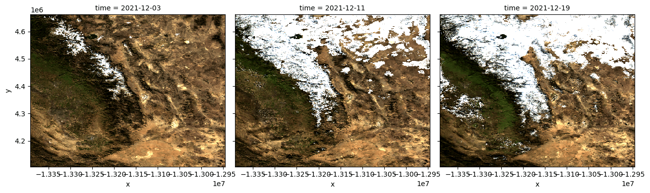
Let's access the Surface Reflectance 8-Day (09A1) data near Mount Whitney in California.

In [3]:

# Mount Whitney in CA
location = shapely.geometry.Point(-118.2923, 36.5785)
bbox = location.buffer(2).bounds
datetimes = [
    "2021-12-03",
    "2021-12-11",
    "2021-12-19",
]

buffer = 2
items = dict()

# Fetch the collection of interest and print available items

for datetime in datetimes:
    print(f"Fetching {datetime}")
    search = catalog.search(
        collections=["modis-09A1-061"],
        intersects=location,
        datetime=datetime,
    )
    items[datetime] = search.item_collection()[0]

print(items)

Fetching 2021-12-03
Fetching 2021-12-11
Fetching 2021-12-19
{'2021-12-03': <Item id=MYD09A1.A2021337.h08v05.061.2021346053944>, '2021-12-11': <Item id=MYD09A1.A2021345.h08v05.061.2021355051559>, '2021-12-19': <Item id=MYD09A1.A2021353.h08v05.061.2022003220209>}

Available Assets¶

Each item has several available assets, including the original HDF file and a Cloud-optimized GeoTIFF of each subdataset.

In [4]:

t = rich.table.Table("Key", "Title")
for key, asset in items["2021-12-03"].assets.items():
    t.add_row(key, asset.title)
t

Out[4]:

┏━━━━━━━━━━━━━━━━━━━━━━┳━━━━━━━━━━━━━━━━━━━━━━━━━━━━━━━━━━━━━━━━━━━━━━━━━━━━━┓
┃ Key                  ┃ Title                                               ┃
┡━━━━━━━━━━━━━━━━━━━━━━╇━━━━━━━━━━━━━━━━━━━━━━━━━━━━━━━━━━━━━━━━━━━━━━━━━━━━━┩
│ hdf                  │ Source data containing all bands                    │
│ metadata             │ Federal Geographic Data Committee (FGDC) Metadata   │
│ sur_refl_b01         │ Surface Reflectance Band 1 (620-670 nm)             │
│ sur_refl_b02         │ Surface Reflectance Band 2 (841-876 nm)             │
│ sur_refl_b03         │ Surface Reflectance Band 3 (459-479 nm)             │
│ sur_refl_b04         │ Surface Reflectance Band 4 (545-565 nm)             │
│ sur_refl_b05         │ Surface Reflectance Band 5 (1230-1250 nm)           │
│ sur_refl_b06         │ Surface Reflectance Band 6 (1628-1652 nm)           │
│ sur_refl_b07         │ Surface Reflectance Band 7 (2105-2155 nm)           │
│ sur_refl_raz         │ MODIS relative azimuth angle                        │
│ sur_refl_szen        │ MODIS solar zenith angle                            │
│ sur_refl_vzen        │ MODIS view zenith angle                             │
│ sur_refl_qc_500m     │ Surface reflectance 500m band quality control flags │
│ sur_refl_state_500m  │ Surface reflectance 500m state flags                │
│ sur_refl_day_of_year │ Day of the year for the pixel                       │
│ tilejson             │ TileJSON with default rendering                     │
│ rendered_preview     │ Rendered preview                                    │
└──────────────────────┴─────────────────────────────────────────────────────┘

Loading the imagery data¶

For this example, we'll visualize the imagery data over Mount Whitney in California. Let's grab each fire mask cover COG and load them into an xarray using odc-stac. The MODIS coordinate reference system is a sinusoidal grid, which means that views in a naïve XY raster look skewed. For visualization purposes, we reproject to a spherical Mercator projection for intuitive, north-up visualization.

In [5]:

RGB = ["sur_refl_b01", "sur_refl_b04", "sur_refl_b03"]

data = odc.stac.load(
    items.values(), crs="EPSG:3857", bbox=bbox, resolution=1000, bands=RGB
)

data

In [6]:

vis = data.odc.to_rgba(RGB, vmin=1, vmax=3000)

Displaying the data¶

Let's display the imagery data.

In [7]:

vis.plot.imshow(col="time", rgb="band", col_wrap=3, robust=True, size=4);

The following snippet will make an interactive slider to control the date visualized

import hvplot.xarray  # noqa: F401

hvplot_kwargs = {
    "frame_width": 250,
    "xaxis": None,
    "yaxis": None,
    "widget_location": "bottom",
    "aspect": len(data.x) / len(data.y),
}

vis.hvplot.rgb("x", "y", bands="band", groupby="time", **hvplot_kwargs)

If you're working in running notebook, that will display a HoloViews plot with an interactive slider to control the date visualized.

User guides¶

MOD09: https://lpdaac.usgs.gov/documents/925/MOD09_User_Guide_V61.pdf