Microsoft Building Footprints Example¶

Bing Maps is releasing open building footprints around the world. The building footprints are detected using Bing Maps imagery between 2014 and 2021 including Maxar and Airbus imagery. The data is freely available for download and use under ODbL.

In [1]:

import planetary_computer
import pystac_client
import deltalake
import shapely.geometry
import contextily
import mercantile

Data access¶

The datasets hosted by the Planetary Computer are available from Azure Blob Storage. We'll use pystac-client to search the Planetary Computer's STAC API to get a link to the assets. We'll specify a modifier so that we can access the data stored in the Planetary Computer's private Blob Storage Containers. See Reading from the STAC API and Using tokens for data access for more.

In [2]:

catalog = pystac_client.Client.open(
    "https://planetarycomputer.microsoft.com/api/stac/v1",
    modifier=planetary_computer.sign_inplace,
)
collection = catalog.get_collection("ms-buildings")

Using Delta Table Files¶

The assets are a set of geoparquet files grouped by a processing date. Newer files (since April 25th, 2023) are stored in Delta Format. This is a layer on top of parquet files offering scalable metadata handling, which is useful for this dataset.

In [3]:

asset = collection.assets["delta"]

This Delta Table is partitioned by RegionName and quadkey. Each (RegionName, quadkey) pair will contain one or more parquet files (depending on how dense that particular quadkey) is. The quadkeys are at level 9 of the Bing Maps Tile System.

In [4]:

storage_options = {
    "account_name": asset.extra_fields["table:storage_options"]["account_name"],
    "sas_token": asset.extra_fields["table:storage_options"]["credential"],
}
table = deltalake.DeltaTable(asset.href, storage_options=storage_options)

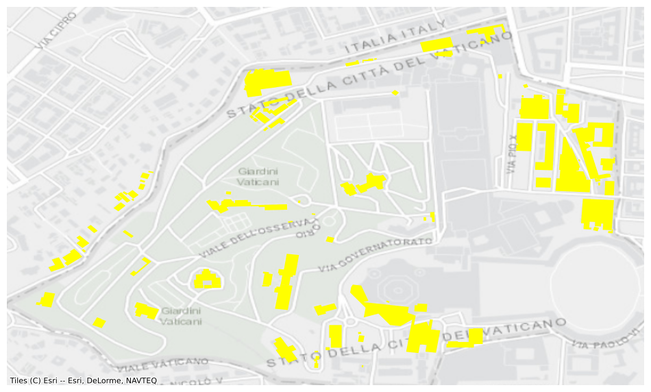
You can load all the files for a given RegionName with a query like this:

In [5]:

import geopandas
import pandas as pd

file_uris = table.file_uris([("RegionName", "=", "VaticanCity")])
df = pd.concat(
    [
        geopandas.read_parquet(file_uri, storage_options=storage_options)
        for file_uri in file_uris
    ]
)

In [6]:

ax = df.plot(figsize=(12, 12), color="yellow")
contextily.add_basemap(
    ax,
    source=contextily.providers.Esri.WorldGrayCanvas,
    crs=df.crs.to_string(),
    zoom=16,
)
ax.set_axis_off()

This partitioning, and the Delta Table format, let you quickly query the subset of files that match your area of interest.

For example, we can visualize the footprints for a small region outside the town of Ueckermünde in Northeast Germany defined by this bounding box.

In [7]:

area_of_interest = shapely.geometry.box(14.11, 53.73, 14.13, 53.75)

You will need to translate your area of interest to a set of intersecting quadkeys, which can be done with mercantile.

In [8]:

quadkeys = [
    int(mercantile.quadkey(tile))
    for tile in mercantile.tiles(*area_of_interest.bounds, zooms=9)
]
quadkeys

Out[8]:

[120210300, 120210302]

Now we can provide those quadkeys as a partition filter to get the set of matching URIs.

In [9]:

uris = table.file_uris([("RegionName", "=", "Germany"), ("quadkey", "in", quadkeys)])
uris

Out[9]:

['az://footprints/delta/2023-04-25/ml-buildings.parquet/RegionName=Germany/quadkey=120210300/part-00168-a20a8489-66de-4ede-be14-48423c230226.c000.snappy.parquet',
 'az://footprints/delta/2023-04-25/ml-buildings.parquet/RegionName=Germany/quadkey=120210302/part-00197-b547555b-9f9e-4cf2-8016-b35087e71f2b.c000.snappy.parquet']

And quickly load them into, for example, a geopandas.GeoDataFrame:

In [10]:

df = pd.concat(
    [
        geopandas.read_parquet(file_uri, storage_options=storage_options)
        for file_uri in uris
    ]
)

Which can be visualized:

In [11]:

subset = df.clip(area_of_interest)
subset.explore()

Out[11]:

Make this Notebook Trusted to load map: File -> Trust Notebook

Using the STAC API¶

As an alternative to Delta, you can use the Planetary Computer STAC API to query files matching your area of interest.

In [12]:

search = catalog.search(
    collections=["ms-buildings"],
    intersects=area_of_interest,
    query={
        "msbuildings:region": {"eq": "Germany"},
        "msbuildings:processing-date": {"eq": "2023-04-25"},
    },
)

ic = search.item_collection()
len(ic)

Out[12]:

See the summaries on the collection for a list of valid processing dates.

Once you have the items, you can load them into a GeoDataFrame. Note that each data asset has one or more parquet files under it, so we need to do two levels of concatentation.

In [13]:

import adlfs

fs = adlfs.AzureBlobFileSystem(
    **ic[0].assets["data"].extra_fields["table:storage_options"]
)

prefixes = [item.assets["data"].href for item in ic]
parts = []
for item in ic:
    parts.extend(fs.ls(item.assets["data"].href))

In [14]:

df = pd.concat(
    [
        geopandas.read_parquet(f"az://{part}", storage_options=storage_options)
        for part in parts
    ]
)
df.head()

Out[14]:

	geometry	meanHeight
0	POLYGON ((14.23111 53.66713, 14.23120 53.66714...	-1.0
1	POLYGON ((14.13342 53.53018, 14.13337 53.53030...	-1.0
2	POLYGON ((14.34231 53.33267, 14.34236 53.33258...	-1.0
3	POLYGON ((14.09257 53.49413, 14.09274 53.49409...	-1.0
4	POLYGON ((14.07604 53.68923, 14.07603 53.68927...	-1.0

Next steps¶

This example briefly demonstrated searching the STAC catalog and loading the data with geopandas. To learn more, visit the following resources:

Learn more about geopandas.
Learn more about Dask
Learn more about geoparquet
Learn more about the Global MLBuildings Footprints project.