Accessing NOAA's Global Ocean Heat Content Climate Data Record (CDR) with the Planetary Computer STAC API¶

The Ocean Heat Content Climate Data Record (CDR) is a set of ocean heat content anomaly (OHCA) time-series for 1955–present on 3-monthly, yearly, and pentadal (five-yearly) scales. This CDR quantifies ocean heat content change over time, which is an essential metric for understanding climate change and the Earth’s energy budget. It provides time-series for multiple depth ranges in the global ocean and each of the major basins (Atlantic, Pacific, and Indian) divided by hemisphere (Northern, Southern).

Data access¶

This notebook works with or without an API key, but you will be given more permissive access to the data with an API key. The Planetary Computer Hub sets the environment variable "PC_SDK_SUBSCRIPTION_KEY" when your server is started. When your Planetary Computer account request was approved, a pair of subscription keys were automatically generated for you. You can view your keys by singing in to the developer portal. The API key may be set manually via the following code:

pc.settings.set_subscription_key(<YOUR API Key>)

The datasets hosted by the Planetary Computer are available from Azure Blob Storage. We'll use pystac-client to search the Planetary Computer's STAC API for the subset of the data that we care about, and then we'll load the data directly from Azure Blob Storage. We'll specify a modifier so that we can access the data stored in the Planetary Computer's private Blob Storage Containers. See Reading from the STAC API and Using tokens for data access for more.

The Ocean Heat Content CDR includes data over multiple time intervals, and for multiple maximum ocean depths. Let's use the Collection summaries to see what values are available.

In [1]:

import planetary_computer
import pystac_client
from rich.table import Table

client = pystac_client.Client.open(
    "https://planetarycomputer.microsoft.com/api/stac/v1",
    modifier=planetary_computer.sign_inplace,
)
collection = client.get_collection(
    "noaa-cdr-ocean-heat-content",
)

table = Table("Key", "Value")
for key, value in collection.summaries.to_dict().items():
    table.add_row(key, str(value))
table

Out[1]:

┏━━━━━━━━━━━━━━━━━━━━┳━━━━━━━━━━━━━━━━━━━━━━━━━━━━━━━━━━━━━━━━━━━━━━━┓
┃ Key                ┃ Value                                         ┃
┡━━━━━━━━━━━━━━━━━━━━╇━━━━━━━━━━━━━━━━━━━━━━━━━━━━━━━━━━━━━━━━━━━━━━━┩
│ noaa_cdr:interval  │ ['monthly', 'seasonal', 'yearly', 'pentadal'] │
│ noaa_cdr:max_depth │ [100, 700, 2000]                              │
└────────────────────┴───────────────────────────────────────────────┘

For this example, let's work with the most recent yearly items with a maximum depth of 700m.

In [2]:

item_search = client.search(
    collections=["noaa-cdr-ocean-heat-content"],
    query={
        "noaa_cdr:interval": {"eq": "yearly"},
        "noaa_cdr:max_depth": {"eq": 700},
    },
    max_items=10,
)
items = list(item_search.items())
items

Out[2]:

[<Item id=ocean-heat-content-2020-700m>,
 <Item id=ocean-heat-content-2019-700m>,
 <Item id=ocean-heat-content-2018-700m>,
 <Item id=ocean-heat-content-2017-700m>,
 <Item id=ocean-heat-content-2016-700m>,
 <Item id=ocean-heat-content-2015-700m>,
 <Item id=ocean-heat-content-2014-700m>,
 <Item id=ocean-heat-content-2013-700m>,
 <Item id=ocean-heat-content-2012-700m>,
 <Item id=ocean-heat-content-2011-700m>]

Assets¶

Each item has a Cloud Optimized GeoTIFF (COG) asset containing several computed values. We'll focus on the heat_content asset for this example.

In [3]:

item = items[0]
table = Table("Key", "Title")
for key, asset in item.assets.items():
    table.add_row(key, asset.title)
table

Out[3]:

┏━━━━━━━━━━━━━━━━━━━━━━━━━━━━━┳━━━━━━━━━━━━━━━━━━━━━━━━━━━━━━━━━━━━━━━━━━━━━━━━━━━━━━━━━━━━━━━━┓
┃ Key                         ┃ Title                                                          ┃
┡━━━━━━━━━━━━━━━━━━━━━━━━━━━━━╇━━━━━━━━━━━━━━━━━━━━━━━━━━━━━━━━━━━━━━━━━━━━━━━━━━━━━━━━━━━━━━━━┩
│ heat_content                │ Ocean Heat Content anomalies from WOA09 : 0-700m 2020          │
│ mean_salinity               │ Mean salinity anomalies from WOA09 : 0-700m 2020               │
│ mean_temperature            │ Mean temperature anomalies from WOA09 : 0-700m 2020            │
│ mean_halosteric_sea_level   │ Mean halosteric sea level anomalies from WOA09 : 0-700m 2020   │
│ mean_thermosteric_sea_level │ Mean thermosteric sea level anomalies from WOA09 : 0-700m 2020 │
│ mean_total_steric_sea_level │ Mean total steric sea level anomalies from WOA09 : 0-700m 2020 │
│ tilejson                    │ TileJSON with default rendering                                │
│ rendered_preview            │ Rendered preview                                               │
└─────────────────────────────┴────────────────────────────────────────────────────────────────┘

Load data¶

Let's load all the data into an xarray using odc-stac.

In [4]:

import odc.stac

data = odc.stac.load(items, bands="heat_content")
data

Visualize¶

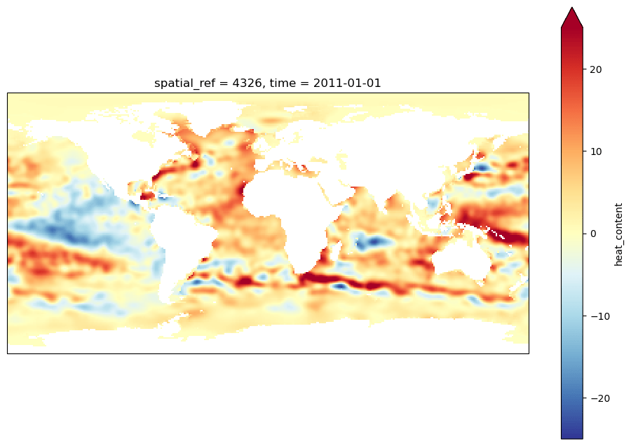
Now, let's visualize one year's heat content.

In [5]:

from cartopy import crs
from matplotlib import pyplot

figure = pyplot.figure(figsize=(12, 8))
axes = pyplot.axes(projection=crs.Mercator())
data["heat_content"][0].plot.imshow(cmap="RdYlBu_r", vmin=-25, vmax=25);

NetCDF data¶

We recommend using the Cloud-Optimized GeoTIFF assets provided by the noaa-cdr-ocean-heat-content collection, but if you'd like to use the source NetCDFs that the COGs were created from, you can as well. Those are stored in the noaa-cdr-ocean-heat-content-netcdf collection.

In [6]:

item_search = client.search(
    collections=["noaa-cdr-ocean-heat-content-netcdf"],
    query={
        "noaa_cdr:interval": {"eq": "monthly"},
        "noaa_cdr:max_depth": {"eq": 2000},
    },
    max_items=10,
)
items = list(item_search.items())
print(items)

[<Item id=heat_content_anomaly_0-2000_monthly>]

You can use xarray (via fsspec) to access the data in the NetCDF.

In [7]:

import fsspec
import xarray
from IPython.display import display

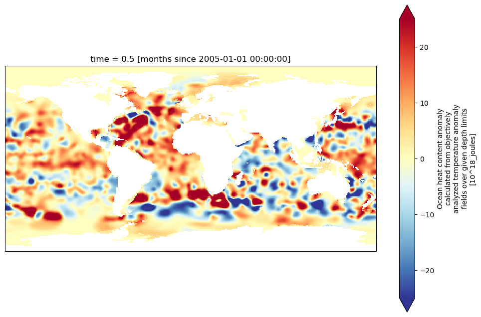
figure = pyplot.figure(figsize=(12, 8))
axes = pyplot.axes(projection=crs.Mercator())
with fsspec.open(items[0].assets["netcdf"].href) as file:
    with xarray.open_dataset(file, decode_times=False) as dataset:
        display(dataset)
        dataset["h18_hc"].isel(time=0).squeeze().plot.imshow(
            cmap="RdYlBu_r", vmin=-25, vmax=25
        )