Accessing NOAA's Sea Surface Temperature - Optimum Interpolation CDR Climate Data Record (CDR) with the Planetary Computer STAC API¶

The NOAA 1/4° daily Optimum Interpolation Sea Surface Temperature (or daily OISST) Climate Data Record (CDR) provides complete ocean temperature fields constructed by combining bias-adjusted observations from different platforms (satellites, ships, buoys) on a regular global grid, with gaps filled in by interpolation. The main input source is satellite data from the Advanced Very High Resolution Radiometer (AVHRR), which provides high temporal-spatial coverage from late 1981-present. This input must be adjusted to the buoys due to erroneous cold SST data following the Mt Pinatubo and El Chichon eruptions. Applications include climate modeling, resource management, ecological studies on annual to daily scales.

Data access¶

This notebook works with or without an API key, but you will be given more permissive access to the data with an API key. The Planetary Computer Hub sets the environment variable "PC_SDK_SUBSCRIPTION_KEY" when your server is started. When your Planetary Computer account request was approved, a pair of subscription keys were automatically generated for you. You can view your keys by singing in to the developer portal. The API key may be set manually via the following code:

pc.settings.set_subscription_key(<YOUR API Key>)

The datasets hosted by the Planetary Computer are available from Azure Blob Storage. We'll use pystac-client to search the Planetary Computer's STAC API for the subset of the data that we care about, and then we'll load the data directly from Azure Blob Storage. We'll specify a modifier so that we can access the data stored in the Planetary Computer's private Blob Storage Containers. See Reading from the STAC API and Using tokens for data access for more.

First, let's fetch all items from the one day in 1981.

In [1]:

import planetary_computer
import pystac_client

client = pystac_client.Client.open(
    "https://planetarycomputer.microsoft.com/api/stac/v1",
    modifier=planetary_computer.sign_inplace,
)
item_search = client.search(
    collections="noaa-cdr-sea-surface-temperature-whoi",
    datetime="1988-01-01T22:00:00Z",
)
item = next(item_search.items())
print(item)

<Item id=SEAFLUX-OSB-CDR_V02R00_SST_D19880101_C20160820-7>

Assets¶

Each item has a Cloud Optimized GeoTIFF (COG) asset containing the sea surface temperature.

In [2]:

from rich.table import Table

table = Table("Key", "Title")
for key, asset in item.assets.items():
    table.add_row(key, asset.title)
table

Out[2]:

┏━━━━━━━━━━━━━━━━━━━━━━━━━┳━━━━━━━━━━━━━━━━━━━━━━━━━━━━━━━━━━━━━┓
┃ Key                     ┃ Title                               ┃
┡━━━━━━━━━━━━━━━━━━━━━━━━━╇━━━━━━━━━━━━━━━━━━━━━━━━━━━━━━━━━━━━━┩
│ fill_missing_qc         │ Quality flag for missing data       │
│ sea_surface_temperature │ NOAA CDR of sea surface temperature │
│ tilejson                │ TileJSON with default rendering     │
│ rendered_preview        │ Rendered preview                    │
└─────────────────────────┴─────────────────────────────────────┘

Load data¶

Let's load all the data into an xarray using odc-stac, converting our nodata values to nan and scaling the data to degrees Celsius.

In [3]:

import odc.stac

data = odc.stac.load([item], bands="sea_surface_temperature")
data

Visualize¶

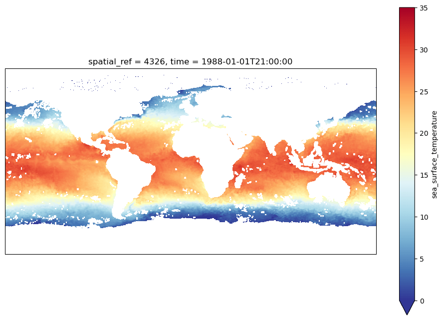
Now, let's visualize one day's data.

In [4]:

from cartopy import crs
from matplotlib import pyplot

figure = pyplot.figure(figsize=(12, 8))
axes = pyplot.axes(projection=crs.Mercator())
data["sea_surface_temperature"][0].plot.imshow(cmap="RdYlBu_r", vmin=0, vmax=35);

NetCDF data¶

We recommend using the Cloud-Optimized GeoTIFF assets provided by the noaa-cdr-sea-surface-temperature-whoi collection, but if you'd like to use the source NetCDFs that the COGs were created from, you can as well. Those are stored in the noaa-cdr-sea-surface-temperature-whoi-netcdf collection.

In [5]:

item_search = client.search(
    collections="noaa-cdr-sea-surface-temperature-whoi-netcdf",
    datetime="1988-01-01T22:00:00Z",
)
item = next(item_search.items())
print(item)

<Item id=SEAFLUX-OSB-CDR_V02R00_SST_D19880101_C20160820>

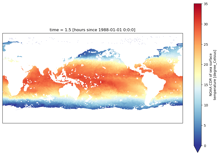
You can use xarray (via fsspec) to access the data in the NetCDF.

In [6]:

import fsspec
import xarray
from IPython.display import display

figure = pyplot.figure(figsize=(12, 8))
axes = pyplot.axes(projection=crs.Mercator())
with fsspec.open(item.assets["netcdf"].href) as file:
    with xarray.open_dataset(file, decode_times=False) as dataset:
        display(dataset)
        dataset["sea_surface_temperature"].isel(time=0).squeeze().plot.imshow(
            cmap="RdYlBu_r", vmin=0, vmax=35
        )