Accessing Sentinel-1 RTC data with the Planetary Computer STAC API¶

The Sentinel 1 RTC product in this collection is a radiometrically terrain corrected product derived from the Sentinel-1 Ground Range Detected (GRD) Level-1 products produced by the European Space Agency.

Environment setup¶

Running this notebook requires an API key.

The Planetary Computer Hub is pre-configured to use your API key.
To use your API key locally, set the environment variable PC_SDK_SUBSCRIPTION_KEY or use planetary_computer.settings.set_subscription_key(<YOUR API Key>)

See when an account is needed for more, and request an account if needed.

In [1]:

import ipyleaflet
import matplotlib.pyplot as plt
import numpy as np
import pystac
import pystac_client
import planetary_computer
import requests
import rich.table

from IPython.display import Image

Data access¶

The datasets hosted by the Planetary Computer are available from Azure Blob Storage. We'll use pystac-client to search the Planetary Computer's STAC API for the subset of the data that we care about, and then we'll load the data directly from Azure Blob Storage. We'll specify a modifier so that we can access the data stored in the Planetary Computer's private Blob Storage Containers. See Reading from the STAC API and Using tokens for data access for more.

In [2]:

catalog = pystac_client.Client.open(
    "https://planetarycomputer.microsoft.com/api/stac/v1",
    modifier=planetary_computer.sign_inplace,
)

Choose an area and time of interest¶

We'll search for assets acquired over Panama in the first week of May, 2022. You can use the Planetary Computer Explorer to find areas of interest.

In [3]:

bbox = [-80.11, 8.71, -79.24, 9.38]
search = catalog.search(
    collections=["sentinel-1-rtc"], bbox=bbox, datetime="2022-05-02/2022-05-09"
)
items = search.item_collection()
print(f"Found {len(items)} items")
item = items[0]

Found 3 items

The rendered_preview asset lets us quickly visualize the data. For Seninel-1 RTC, this produces a false-color composite from a combination of the VV and VH bands.

In [4]:

Image(url=item.assets["rendered_preview"].href)

Out[4]:

Inspect the STAC metadata¶

The STAC metadata includes many useful pieces of metadata, including metadata from the SAR and Satellite extensions.

In [5]:

table = rich.table.Table("key", "value")
for k, v in sorted(item.properties.items()):
    table.add_row(k, str(v))

table

Out[5]:

┏━━━━━━━━━━━━━━━━━━━━━━━━━━━━━━━━━━━━━━━┳━━━━━━━━━━━━━━━━━━━━━━━━━━━━━━━━━━━━━━━━━━━━━━━━━━━━━━━━━━━━━┓
┃ key                                   ┃ value                                                       ┃
┡━━━━━━━━━━━━━━━━━━━━━━━━━━━━━━━━━━━━━━━╇━━━━━━━━━━━━━━━━━━━━━━━━━━━━━━━━━━━━━━━━━━━━━━━━━━━━━━━━━━━━━┩
│ constellation                         │ Sentinel-1                                                  │
│ datetime                              │ 2022-05-04T23:32:10.313109Z                                 │
│ end_datetime                          │ 2022-05-04 23:32:22.812028+00:00                            │
│ platform                              │ SENTINEL-1A                                                 │
│ proj:bbox                             │ [519450.0, 935520.0, 800080.0, 1153060.0]                   │
│ proj:epsg                             │ 32617                                                       │
│ proj:shape                            │ [28806, 21907]                                              │
│ proj:transform                        │ [10.0, 0.0, 519430.0, 0.0, -10.0, 1154570.0, 0.0, 0.0, 1.0] │
│ s1:datatake_id                        │ 337052                                                      │
│ s1:instrument_configuration_ID        │ 7                                                           │
│ s1:orbit_source                       │ RESORB                                                      │
│ s1:processing_level                   │ 1                                                           │
│ s1:product_timeliness                 │ Fast-24h                                                    │
│ s1:resolution                         │ high                                                        │
│ s1:shape                              │ [28806, 21907]                                              │
│ s1:slice_number                       │ 2                                                           │
│ s1:total_slices                       │ 29                                                          │
│ sar:center_frequency                  │ 5.405                                                       │
│ sar:frequency_band                    │ C                                                           │
│ sar:instrument_mode                   │ IW                                                          │
│ sar:looks_azimuth                     │ 1                                                           │
│ sar:looks_equivalent_number           │ 4.4                                                         │
│ sar:looks_range                       │ 5                                                           │
│ sar:observation_direction             │ right                                                       │
│ sar:pixel_spacing_azimuth             │ 10                                                          │
│ sar:pixel_spacing_range               │ 10                                                          │
│ sar:polarizations                     │ ['VV', 'VH']                                                │
│ sar:product_type                      │ GRD                                                         │
│ sar:resolution_azimuth                │ 22                                                          │
│ sar:resolution_range                  │ 20                                                          │
│ sat:absolute_orbit                    │ 43068                                                       │
│ sat:orbit_state                       │ ascending                                                   │
│ sat:platform_international_designator │ 2014-016A                                                   │
│ sat:relative_orbit                    │ 121                                                         │
│ start_datetime                        │ 2022-05-04 23:31:57.814190+00:00                            │
└───────────────────────────────────────┴─────────────────────────────────────────────────────────────┘

The data assets on every Sentinel-1 RTC item will be some combination of hh, hv, vh, and vv. These represent the terrain-corrected gamma nought values of a signal transmitted in one polarization ("h" or "v") and received in another ("h" or "v"). The sar:polarizations field indicates which assets are available.

In [6]:

item.properties["sar:polarizations"]

Out[6]:

['VV', 'VH']

Visualize the assets¶

Next, we'll load the vv data into xarray and plot the results. We'll use Dask to load the data in parallel. We're working with a small amount of data so we'll use a single machine. For larger datasets, see Scaling with Dask.

In [7]:

from distributed import Client

client = Client(processes=False)
print(client.dashboard_link)

/user/taugspurger@microsoft.com/proxy/8787/status

In [8]:

import stackstac

ds = stackstac.stack(items, bounds_latlon=bbox, epsg=32630, resolution=100)
ds

Out[8]:

<xarray.DataArray 'stackstac-50b066be198a039bc4e73aa60a5208bd' (time: 3,
                                                                band: 2,
                                                                y: 4248, x: 4431)>
dask.array<fetch_raster_window, shape=(3, 2, 4248, 4431), dtype=float64, chunksize=(1, 1, 1024, 1024), chunktype=numpy.ndarray>
Coordinates: (12/39)
  * time                                   (time) datetime64[ns] 2022-05-04T1...
    id                                     (time) <U66 'S1A_IW_GRDH_1SDV_2022...
  * band                                   (band) <U2 'vh' 'vv'
  * x                                      (x) float64 -1.225e+07 ... -1.18e+07
  * y                                      (y) float64 4.171e+06 ... 3.746e+06
    sat:absolute_orbit                     (time) int64 43060 43068 43068
    ...                                     ...
    sar:pixel_spacing_azimuth              int64 10
    sar:resolution_azimuth                 int64 22
    title                                  (band) <U41 'VH: vertical transmit...
    raster:bands                           object {'nodata': -32768, 'data_ty...
    description                            (band) <U173 'Terrain-corrected ga...
    epsg                                   int64 32630
Attributes:
    spec:        RasterSpec(epsg=32630, bounds=(-12247900, 3746300, -11804800...
    crs:         epsg:32630
    transform:   | 100.00, 0.00,-12247900.00|\n| 0.00,-100.00, 4171100.00|\n|...
    resolution:  100

We'll select the vv band for the first timestep found by our search.

In [9]:

vv = ds.sel(band="vv")[0].compute()

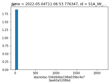
The distribution of the raw values is quite skewed:

In [10]:

vv.plot.hist(bins=30);

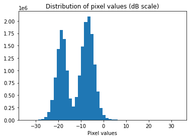
So the values are typically transformed before visualization:

In [11]:

fig, ax = plt.subplots(figsize=(6, 4))

def db_scale(x):
    return 10 * np.log10(x)

db_scale(vv).plot.hist(bins=50, ax=ax)
ax.set(title="Distribution of pixel values (dB scale)", xlabel="Pixel values");

In [12]:

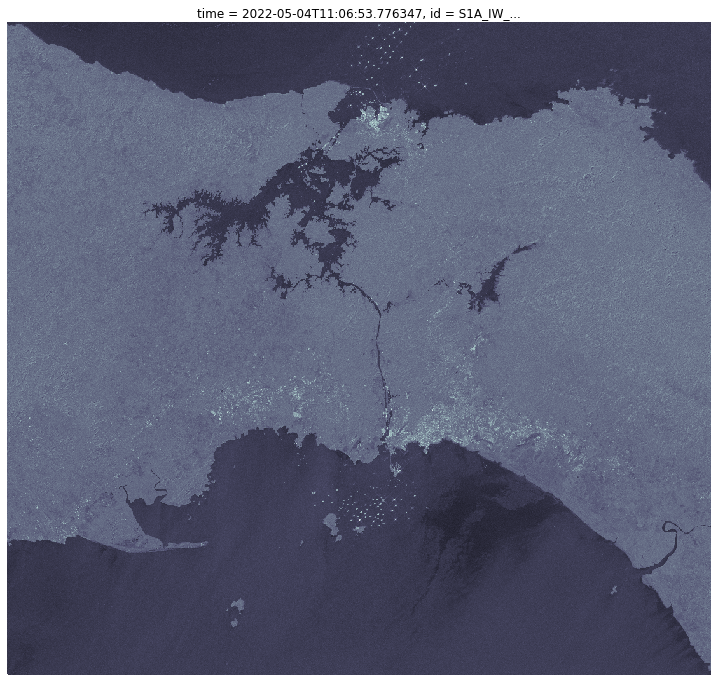
img = (
    db_scale(vv)
    .coarsen(x=4, y=4, boundary="trim")
    .max()
    .plot.imshow(cmap="bone", size=12, aspect=1.05, add_colorbar=False)
)
img.axes.set_axis_off();

The effect of terrain correction¶

In this section, we compare Sentinel-1 GRD to Sentinel-1 RTC to see the effect of terrain correction.

Every Sentinel-1-RTC item is derived from a Sentinel-1-GRD item. You can follow the derived_from link to get back to the original GRD item.

In [13]:

rtc_item = catalog.get_collection("sentinel-1-rtc").get_item(
    "S1A_IW_GRDH_1SDV_20220518T054334_20220518T054359_043261_052A9D_rtc"
)
grd_item = pystac.read_file(rtc_item.get_single_link("derived_from").target)

Next, we'll use the tilejson asset, which uses the Planetary Computer's Data API to serve xyz tiles for a STAC item.

In [14]:

grd_tiles = requests.get(grd_item.assets["tilejson"].href).json()["tiles"][0]
rtc_tiles = requests.get(rtc_item.assets["tilejson"].href).json()["tiles"][0]

With these URLs, we can build an interactive map using ipyleaflet. Adjust the slider to visualize either GRD (to the left) or RTC (to the right).

In [15]:

center = [47.05, 7.10]
m = ipyleaflet.Map(
    center=center,
    zoom=14,
    controls=[ipyleaflet.FullScreenControl()],
)
grd_layer = ipyleaflet.TileLayer(url=grd_tiles)
rtc_layer = ipyleaflet.TileLayer(url=rtc_tiles)

control = ipyleaflet.SplitMapControl(left_layer=grd_layer, right_layer=rtc_layer)
m.add_control(control)
m.scroll_wheel_zoom = True
m

Map(center=[47.05, 7.1], controls=(FullScreenControl(options=['position']), ZoomControl(options=['position', '…

Notice that points seem to "jump" between the GRD and RTC. The RTC values are corrected to align with where they're actually at on the Earth.

For more background on terrain correction, and for an introduction to the sarsen package which enables customizable RTCs, see Sentinel-1 Customizable Radiometric Terrain Correction.