Accessing Sentinel-3 SLSTR data with the Planetary Computer STAC API¶

The Sentinel 3 SLSTR instrument is a Along-Track Scanning Radiometer (ATSR) designed to provide reference land surface and sea surface temperatures. There are three SLSTR collections in the Plantery Computer:

Fire radiative power: sentinel-3-slstr-frp-l2-netcdf
Land surface temperature: sentinel-3-slstr-lst-l2-netcdf
Water surface temperature: sentinel-3-slstr-wst-l2-netcdf

This notebook demonstrates accessing and visualizing data from all three collections.

Data Access¶

This notebook works with or without an API key, but you will be given more permissive access to the data with an API key. If you are using the Planetary Computer Hub to run this notebook, then your API key is automatically set to the environment variable PC_SDK_SUBSCRIPTION_KEY for you when your server is started. Otherwise, you can view your keys by signing in to the developer portal. The API key may be manually set via the environment variable PC_SDK_SUBSCRIPTION_KEY or the following code:

import planetary_computer
planetary_computer.settings.set_subscription_key(<YOUR API Key>)

The datasets hosted by the Planetary Computer are available in Azure Blob Storage. We'll use pystac-client to search the Planetary Computer's STAC API for the subset of the data that we care about, and then we'll load the data directly from Azure Blob Storage. We'll specify a modifier so that we can access the data stored in the Planetary Computer's private Blob Storage Containers. See Reading from the STAC API and Using tokens for data access for more.

Land surface temperature¶

The collection's description provides more information about the LST product.

In [1]:

import planetary_computer
import pystac_client
from IPython.display import display, Markdown

catalog = pystac_client.Client.open(
    "https://planetarycomputer.microsoft.com/api/stac/v1",
    modifier=planetary_computer.sign_inplace,
)
collection = catalog.get_collection("sentinel-3-slstr-lst-l2-netcdf")

display(Markdown(f"### {collection.id}\n\n{collection.description}"))

sentinel-3-slstr-lst-l2-netcdf¶

This Collection provides Sentinel-3 SLSTR Level-2 Land Surface Temperature products containing data on land surface temperature measurements on a 1km grid. Radiance is measured in two channels to determine the temperature of the Earth's surface skin in the instrument field of view, where the term "skin" refers to the top surface of bare soil or the effective emitting temperature of vegetation canopies as viewed from above.

Data files¶

The dataset includes data on the primary measurement variable, land surface temperature, in a single NetCDF file, LST_in.nc. A second file, LST_ancillary.nc, contains several ancillary variables:

Normalized Difference Vegetation Index
Surface biome classification
Fractional vegetation cover
Total water vapor column

In addition to the primary and ancillary data files, a standard set of annotation data files provide meteorological information, geolocation and time coordinates, geometry information, and quality flags. More information about the product and data processing can be found in the User Guide and Technical Guide.

This Collection contains Level-2 data in NetCDF files from April 2016 to present.

STAC Item geometries¶

The Collection contains small "chips" and long "stripes" of data collected along the satellite direction of travel. Approximately five percent of the STAC Items describing long stripes of data contain geometries that encompass a larger area than an exact concave hull of the data extents. This may require additional filtering when searching the Collection for Items that spatially intersect an area of interest.

Define the area of interest and search the land surface temperature collection¶

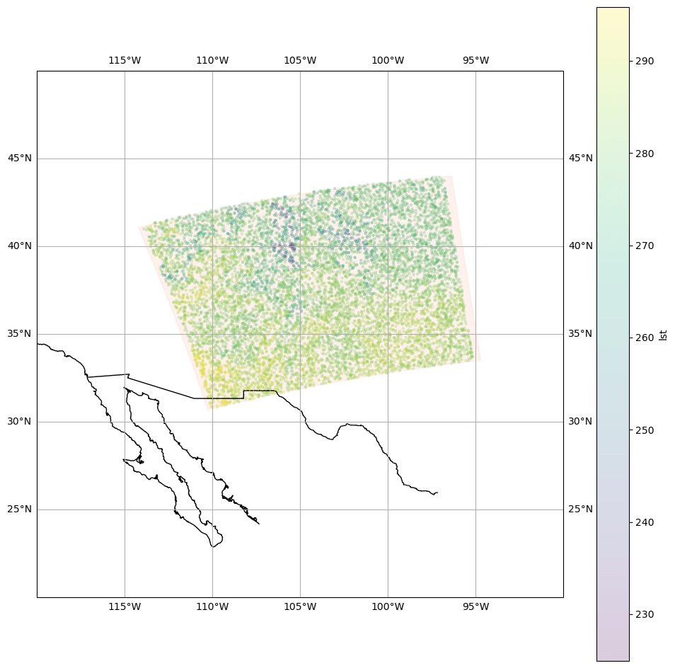
We'll search for items over the coordinates [-105, 40].

In [2]:

import xarray as xr
import fsspec

search = catalog.search(
    collections=["sentinel-3-slstr-lst-l2-netcdf"],
    intersects={"type": "Point", "coordinates": [-105, 40]},
)
item = next(search.items())

Available Assets and Metadata¶

Each item includes a handful of assets linking to NetCDF files with the data or additional metadata files.

In [3]:

import rich.table

t = rich.table.Table("Key", "Value")
for key, asset in item.assets.items():
    t.add_row(key, asset.description)

t

Out[3]:

┏━━━━━━━━━━━━━━━━━━━━┳━━━━━━━━━━━━━━━━━━━━━━━━━━━━━━━━━━━━━━━━━━━━━━━━━━━━━━━━━━━━━━━━━━━━━━━━━━━━━━━┓
┃ Key                ┃ Value                                                                         ┃
┡━━━━━━━━━━━━━━━━━━━━╇━━━━━━━━━━━━━━━━━━━━━━━━━━━━━━━━━━━━━━━━━━━━━━━━━━━━━━━━━━━━━━━━━━━━━━━━━━━━━━━┩
│ lst-in             │ Land Surface Temperature (LST) values                                         │
│ slstr-met-tx       │ Meteorological parameters regridded onto the 16km tie points                  │
│ safe-manifest      │ SAFE product manifest                                                         │
│ slstr-time-in      │ Time annotations for the 1km grid                                             │
│ slstr-flags-in     │ Global flags for the 1km TIR grid, nadir view                                 │
│ lst-ancillary-ds   │ LST ancillary measurement dataset                                             │
│ slstr-indices-in   │ Scan, pixel and detector indices annotations for the 1km TIR grid, nadir view │
│ slstr-geodetic-in  │ Full resolution geodetic coordinates for the 1km TIR grid, nadir view         │
│ slstr-geodetic-tx  │ 16km geodetic coordinates                                                     │
│ slstr-geometry-tn  │ 16km solar and satellite geometry annotations, nadir view                     │
│ slstr-cartesian-in │ Full resolution cartesian coordinates for the 1km TIR grid, nadir view        │
│ slstr-cartesian-tx │ 16km cartesian coordinates                                                    │
└────────────────────┴───────────────────────────────────────────────────────────────────────────────┘

Reading data¶

We can use xarray to read each NetCDF file directly from Blob Storage.

In [4]:

dataset = xr.open_dataset(fsspec.open(item.assets["lst-in"].href).open())
dataset

Geolocating and subsetting the data¶

To plot the land surface temperature data, we will use the georeferencing information contained in the slstr-geodetic-in asset. There's so many points, and the data have such a large spatial extent, that we only need a random sample of the data rather than every point.

In [5]:

geo = xr.open_dataset(fsspec.open(item.assets["slstr-geodetic-in"].href).open()).load()
geo

In [6]:

import pandas

data = (
    pandas.DataFrame(
        {
            "longitude": geo.longitude_in.data.ravel(),
            "latitude": geo.latitude_in.data.ravel(),
            "lst": dataset.LST.load().data.ravel(),
        }
    )
    .dropna()
    .sample(10000)
)
data

Out[6]:

	longitude	latitude	lst
1020954	-106.477214	37.928197	274.365997
1210376	-111.487024	38.031391	272.294006
1078016	-107.259553	38.127250	274.444000
861178	-97.549408	38.335761	276.816010
1055490	-106.929072	38.053571	267.406006
...	...	...	...
424405	-110.153256	33.394046	287.675995
371951	-110.523054	32.971659	292.160004
1170842	-105.485691	39.043829	245.289993
255360	-98.851436	34.515057	283.153992
1175948	-112.193523	37.647869	278.306000

10000 rows × 3 columns

Plotting land surface temperature data¶

We use a scatter plot to visualize the land surface temperature points over the globe. We also plot the item geometry, to give us a sense of the satellite's field of view and where that field of view crosses the land.

In [7]:

import shapely.geometry
from cartopy.crs import PlateCarree
from cartopy.feature import BORDERS
import matplotlib.pyplot as plt

fig, ax = plt.subplots(figsize=(12, 12), subplot_kw=dict(projection=PlateCarree()))

ax.add_geometries(
    shapely.geometry.shape(item.geometry), crs=PlateCarree(), color="coral", alpha=0.1
)

data.plot.scatter(
    x="longitude",
    y="latitude",
    c="lst",
    ax=ax,
    colormap="viridis",
    marker=".",
    alpha=0.2,
)
ax.set(ybound=(20, 50), xbound=(-120, -90))
ax.coastlines()
ax.add_feature(BORDERS, linestyle="-")
ax.gridlines(draw_labels=True, dms=True, x_inline=False, y_inline=False);

Water surface temperature data¶

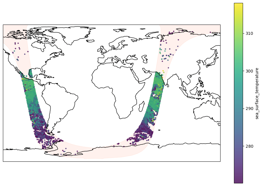
Let's do the same process, but for the water surface temperature product. The data structure is a little different.

In [8]:

collection = catalog.get_collection("sentinel-3-slstr-wst-l2-netcdf")

display(Markdown(f"### {collection.id}\n\n{collection.description}"))

sentinel-3-slstr-wst-l2-netcdf¶

This Collection provides Sentinel-3 SLSTR Level-2 Water Surface Temperature products containing data on sea surface temperature measurements on a 1km grid. Each product consists of a single NetCDF file containing all data variables:

Sea Surface Temperature (SST) value
SST total uncertainty
Latitude and longitude coordinates
SST time deviation
Single Sensor Error Statistic (SSES) bias and standard deviation estimate
Contextual parameters such as wind speed at 10 m and fractional sea-ice contamination
Quality flag
Satellite zenith angle
Top Of Atmosphere (TOA) Brightness Temperature (BT)
TOA noise equivalent BT

More information about the product and data processing can be found in the User Guide and Technical Guide.

This Collection contains Level-2 data in NetCDF files from October 2017 to present.

In [9]:

search = catalog.search(
    collections=["sentinel-3-slstr-wst-l2-netcdf"],
    intersects={"type": "Point", "coordinates": [-105, 40]},
)
item = next(search.items())
t = rich.table.Table("Key", "Value")
for key, asset in item.assets.items():
    t.add_row(key, asset.description)

t

Out[9]:

┏━━━━━━━━━━━━━━━┳━━━━━━━━━━━━━━━━━━━━━━━━━━━━━━━━━━━━━━━━━━━━━━━━━━━━━━━━━━━━━━━━━━━━━━━━━━━━━━━━━━━━━━━━━━━━━━━━━┓
┃ Key           ┃ Value                                                                                           ┃
┡━━━━━━━━━━━━━━━╇━━━━━━━━━━━━━━━━━━━━━━━━━━━━━━━━━━━━━━━━━━━━━━━━━━━━━━━━━━━━━━━━━━━━━━━━━━━━━━━━━━━━━━━━━━━━━━━━━┩
│ l2p           │ Skin Sea Surface Temperature (SST) values                                                       │
│ browse-jpg    │ Preview image produced by the European Organisation for the Exploitation of Meteorological      │
│               │ Satellites (EUMETSAT)                                                                           │
│ eop-metadata  │ Metadata produced by the European Organisation for the Exploitation of Meteorological           │
│               │ Satellites (EUMETSAT)                                                                           │
│ safe-manifest │ SAFE product manifest                                                                           │
└───────────────┴─────────────────────────────────────────────────────────────────────────────────────────────────┘

In [10]:

dataset = xr.open_dataset(fsspec.open(item.assets["l2p"].href).open())
dataset

In [11]:

import pandas

data = (
    pandas.DataFrame(
        {
            "longitude": dataset.lon.data.ravel(),
            "latitude": dataset.lat.data.ravel(),
            "sea_surface_temperature": dataset.sea_surface_temperature.load().data.ravel(),
        }
    )
    .dropna()
    .sample(10000)
)
data

Out[11]:

	longitude	latitude	sea_surface_temperature
14291493	-97.294258	-5.197991	300.820007
42867585	68.544571	15.891827	303.279999
5517750	-77.549706	-55.720612	279.479980
54869107	46.689182	-54.085552	272.519989
8737663	-80.118530	-35.690479	286.100006
...	...	...	...
17576687	-103.380623	13.824631	302.320007
47112414	61.504601	-8.788809	302.169983
17712804	-100.103874	15.390665	301.239990
5239043	-81.084801	-58.172470	281.130005
53278673	46.693626	-43.741562	280.130005

10000 rows × 3 columns

In [12]:

figure, axes = plt.subplots(figsize=(12, 8), subplot_kw=dict(projection=PlateCarree()))

axes.add_geometries(
    shapely.geometry.shape(item.geometry), crs=PlateCarree(), color="coral", alpha=0.1
)

data.plot.scatter(
    x="longitude",
    y="latitude",
    c="sea_surface_temperature",
    ax=axes,
    colormap="viridis",
    marker=".",
    alpha=0.8,
)
axes.coastlines();

Fire radiative power¶

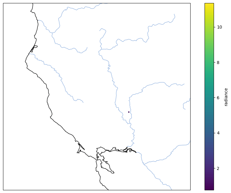
We'll do the same for fire radiative power. This product's items are smaller chips. Let's use an item that crosses over California to give ourselves the best chance of catching data of interest.

In [13]:

collection = catalog.get_collection("sentinel-3-slstr-frp-l2-netcdf")

display(Markdown(f"### {collection.id}\n\n{collection.description}"))

sentinel-3-slstr-frp-l2-netcdf¶

This Collection provides Sentinel-3 SLSTR Level-2 Fire Radiative Power (FRP) products containing data on fires detected over land and ocean.

Data files¶

The primary measurement data is contained in the FRP_in.nc file and provides FRP and uncertainties, projected onto a 1km grid, for fires detected in the thermal infrared (TIR) spectrum over land. Since February 2022, FRP and uncertainties are also provided for fires detected in the short wave infrared (SWIR) spectrum over both land and ocean, with the delivered data projected onto a 500m grid. The latter SWIR-detected fire data is only available for night-time measurements and is contained in the FRP_an.nc or FRP_bn.nc files.

In addition to the measurement data files, a standard set of annotation data files provide meteorological information, geolocation and time coordinates, geometry information, and quality flags.

Processing¶

The TIR fire detection is based on measurements from the S7 and F1 bands of the SLSTR instrument; SWIR fire detection is based on the S5 and S6 bands. More information about the product and data processing can be found in the User Guide and Technical Guide.

This Collection contains Level-2 data in NetCDF files from August 2020 to present.

In [14]:

search = catalog.search(
    collections=["sentinel-3-slstr-frp-l2-netcdf"],
    intersects={"type": "Point", "coordinates": [-121, 40]},
)
item = next(search.items())
t = rich.table.Table("Key", "Value")
for key, asset in item.assets.items():
    t.add_row(key, asset.description)

t

Out[14]:

┏━━━━━━━━━━━━━━━━━━━━┳━━━━━━━━━━━━━━━━━━━━━━━━━━━━━━━━━━━━━━━━━━━━━━━━━━━━━━━━━━━━━━━━━━━━━━━━┓
┃ Key                ┃ Value                                                                  ┃
┡━━━━━━━━━━━━━━━━━━━━╇━━━━━━━━━━━━━━━━━━━━━━━━━━━━━━━━━━━━━━━━━━━━━━━━━━━━━━━━━━━━━━━━━━━━━━━━┩
│ frp-in             │ Fire Radiative Power (FRP) dataset                                     │
│ slstr-met-tx       │ Meteorological parameters regridded onto the 16km tie points           │
│ safe-manifest      │ SAFE product manifest                                                  │
│ slstr-time-in      │ Time annotations for the 1 KM grid                                     │
│ slstr-flags-fn     │ Global flags for the 1km F1 grid, nadir view                           │
│ slstr-flags-in     │ Global flags for the 1km TIR grid, nadir view                          │
│ slstr-indices-fn   │ Scan, pixel and detector annotations for the 1km F1 grid, nadir view   │
│ slstr-indices-in   │ Scan, pixel and detector annotations for the 1km TIR grid, nadir view  │
│ slstr-geodetic-fn  │ Full resolution geodetic coordinates for the 1km F1 grid, nadir view   │
│ slstr-geodetic-in  │ Full resolution geodetic coordinates for the 1km TIR grid, nadir view  │
│ slstr-geodetic-tx  │ 16km geodetic coordinates                                              │
│ slstr-geometry-tn  │ 16km solar and satellite geometry annotations, nadir view              │
│ slstr-cartesian-fn │ Full resolution cartesian coordinates for the 1km F1 grid, nadir view  │
│ slstr-cartesian-in │ Full resolution cartesian coordinates for the 1km TIR grid, nadir view │
│ slstr-cartesian-tx │ 16km cartesian coordinates                                             │
└────────────────────┴────────────────────────────────────────────────────────────────────────┘

In [15]:

dataset = xr.open_dataset(fsspec.open(item.assets["frp-in"].href).open())
dataset

In [16]:

import pandas

data = pandas.DataFrame(
    {
        "longitude": dataset.longitude.data.ravel(),
        "latitude": dataset.latitude.data.ravel(),
        "radiance": dataset.F1_Fire_pixel_radiance.load().data.ravel(),
    }
).dropna()
data

Out[16]:

	longitude	latitude	radiance
0	-113.659809	39.688016	0.918481
1	-111.476330	38.801270	11.352760
2	-111.464705	38.799932	2.332020
3	-118.064226	39.264368	1.464294
4	-121.641641	39.083807	1.075822
...	...	...	...
83	-114.843571	33.928673	1.640789
84	-114.845418	33.919861	1.625753
85	-114.835000	33.917116	1.606819
86	-110.983447	29.555228	2.122387
87	-110.988771	29.546035	2.029452

88 rows × 3 columns

In [17]:

from cartopy.feature import RIVERS, COASTLINE

figure, axes = plt.subplots(figsize=(12, 8), subplot_kw=dict(projection=PlateCarree()))

axes.add_feature(RIVERS)
axes.add_feature(COASTLINE)
data.plot.scatter(
    x="longitude", y="latitude", c="radiance", ax=axes, colormap="viridis", marker="."
)
axes.set_extent((-125, -120, 37, 42));