Notebook

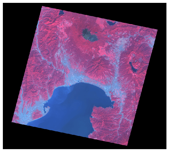
Accessing ASTER L1T data with the Planetary Computer STAC API¶

The ASTER instrument, launched on-board NASA's Terra satellite in 1999, provides multispectral images of the Earth at 15m-90m resolution. ASTER images provide information about land surface temperature, color, elevation, and mineral composition.

This dataset represents ASTER L1T data from 2000-2006. L1T images have been terrain-corrected and rotated to a north-up UTM projection. Data are in cloud-optimized GeoTIFF format.

This notebook demonstrates the use of the Planetary Computer STAC API to query for ASTER scenes.

Environment setup¶

This notebook works with or without an API key, but you will be given more permissive access to the data with an API key. The Planetary Computer Hub is pre-configured to use your API key.

In [1]:

import pystac_client
import planetary_computer
from pystac.extensions.eo import EOExtension as eo

# Set the environment variable PC_SDK_SUBSCRIPTION_KEY, or set it here.
# The Hub sets PC_SDK_SUBSCRIPTION_KEY automatically.
# pc.settings.set_subscription_key(<YOUR API Key>)

Open and explore the ASTER collection¶

The datasets hosted by the Planetary Computer are available from Azure Blob Storage. We'll use pystac-client to search the Planetary Computer's STAC API for the subset of the data that we care about, and then we'll load the data directly from Azure Blob Storage. We'll specify a modifier so that we can access the data stored in the Planetary Computer's private Blob Storage Containers. See Reading from the STAC API and Using tokens for data access for more.

In [2]:

catalog = pystac_client.Client.open(
    "https://planetarycomputer.microsoft.com/api/stac/v1",
    modifier=planetary_computer.sign_inplace,
)
aster_l1t = catalog.get_child(id="aster-l1t")

Let's look at the temporal extent of the collection; the Planetary Computer ASTER L1T dataset contains images from 2000 to 2006:

In [3]:

aster_l1t.extent.temporal.to_dict()

Out[3]:

{'interval': [['2000-03-04T12:00:00Z', '2006-12-31T12:00:00Z']]}

Choose a region and time of interest¶

For this example we'll search 2002 imagery over an area in Japan:

In [4]:

time_of_interest = "2002-01-01/2002-12-31"

area_of_interest = {
    "type": "Polygon",
    "coordinates": [
        [
            [138.4222412109375, 34.90620544067929],
            [138.58428955078125, 34.90620544067929],
            [138.58428955078125, 35.07271701786369],
            [138.4222412109375, 35.07271701786369],
            [138.4222412109375, 34.90620544067929],
        ]
    ],
}

Search the collection and explore the results¶

We'll use this criteria to perform a search against the STAC API:

In [5]:

search = catalog.search(
    collections=["aster-l1t"],
    intersects=area_of_interest,
    datetime=time_of_interest,
    query={"eo:cloud_cover": {"lt": 10}},
)

# Check how many items were returned
items = list(search.get_items())
print(f"Returned {len(items)} Items")

Returned 3 Items

Each of those Item objects represents one ASTER scene. Let's see what assets are available for each ASTER scene:

In [6]:

available_assets = list(aster_l1t.extra_fields["item_assets"].keys())
print(available_assets)

['TIR', 'xml', 'SWIR', 'VNIR', 'qa-txt', 'qa-browse', 'tir-browse', 'vnir-browse']

Render a thumbnail image¶

ASTER data includes thumbnail images in the 'tir-browse' and 'vnir-browse' assets attached to each item. Let's render one of those thumbnails.

Each Item has an href field containing a URL to the underlying image. For ASTER, these URLs are publicly-accessible, but for some data sets, these URLs may point to private containers, so we demonstrate the use of the planetary-computer package's pc.sign method, which adds a Shared Access Signature to the URL, after which it can be used by any tooling that expects a standard URL.

In [7]:

# from PIL import Image
# from urllib.request import urlopen
from IPython.display import Image

# Grab the last item and create an instance of the Electro-Optical (eo)
# extension to check cloud cover
item = items[-1]
item_eo = eo.ext(item)

asset_href = item.assets["vnir-browse"].href

print(f"id={item.id}\tdate={item.datetime.date()}\tcloud %={item_eo.cloud_cover}")

# Downsample a bit for plotting
# image = Image.open(urlopen(asset_href))
# image.resize(size=(image.width // 2, image.height // 2))
Image(url=asset_href)

id=AST_L1T_00310042002014048_20150425134514	date=2002-10-04	cloud %=1.0

Out[7]:

Render an RGB composite from a complete scene¶

Of course, most of the time, you don't just want to browse thumbnails, you want to access images. Let's render a composite image from the VNIR bands in one of the items.

In [8]:

item = min(items, key=lambda item: eo.ext(item).cloud_cover)
swir_asset = item.assets["VNIR"]

Let's see what properties are available within each asset. We'll use the eo extension to print the bands available in this image:

In [9]:

available_assets = list(swir_asset.to_dict().keys())
print("properties:", available_assets)

available_bands = [band.name for band in eo.ext(swir_asset).bands]
print("bands:", available_bands)

properties: ['href', 'type', 'title', 'eo:bands', 'proj:bbox', 'proj:shape', 'proj:transform', 'roles']
bands: ['VNIR_Band1', 'VNIR_Band2', 'VNIR_Band3N']

Finally, let's render our RGB composite.

In [10]:

import numpy as np
import rasterio
import matplotlib.pyplot as plt

# Downsample the scene for plotting
dsfactor = 10

# Choose bands for our RGB composite
bands = [3, 2, 1]

# Normalization value for rendering
norm_value = 100

image_data = []

with rasterio.open(swir_asset.href, "r") as src:

    h = int(src.height // dsfactor)
    w = int(src.width // dsfactor)

    for i, band in enumerate(bands):
        band_array = src.read(band, out_shape=(1, h, w))
        band_array = band_array / norm_value
        image_data.append(band_array)
    src.close()

rgb = np.dstack((image_data[0], image_data[1], image_data[2]))
np.clip(rgb, 0, 1, rgb)

dpi = 100
fig = plt.figure(frameon=False, figsize=(w / dpi, h / dpi), dpi=dpi)
ax = plt.Axes(fig, [0.0, 0.0, 1.0, 1.0])
ax.set_axis_off()
fig.add_axes(ax)
plt.imshow(rgb);