Accessing ECMWF Open Data – Real Time¶

The Planetary Computer includes data from the ECMWF Open Data (real time) program. See the dataset page and ECMWF Uesr Guide for more.

Each item in this collection includes metadata about the stream (or forecasting system) and type that produced that particular dataset. Filter on these values to select the item of interest. For example, we can select data from the wave stream, with the fc type that are forecast 0h hours out.

In [ ]:

import pystac_client
import planetary_computer

catalog = pystac_client.Client.open(
    "https://planetarycomputer.microsoft.com/api/stac/v1",
    modifier=planetary_computer.sign_inplace,
)
search = catalog.search(
    collections=["ecmwf-forecast"],
    query={
        "ecmwf:stream": {"eq": "wave"},
        "ecmwf:type": {"eq": "fc"},
        "ecmwf:step": {"eq": "0h"},
    },
)
items = search.get_all_items()
len(items)

We'll select the most recent item, using the item's datetime.

In [2]:

item = max(items, key=lambda item: item.datetime)
item

Out[2]:

<Item id=ecmwf-2022-03-10T00-wave-fc-0h>

This STAC item has two assets. One asset is the actual GRIB2 file with the data. The second asset is the "index" file, which contains information about the messages within the GRIB2 file.

In [3]:

url = item.assets["data"].href
url

Out[3]:

'https://ai4edataeuwest.blob.core.windows.net/ecmwf/20220310/00z/0p4-beta/wave/20220310000000-0h-wave-fc.grib2'

To open the file with xarray, we can download it locally and open it with cfgrib.

In [4]:

import urllib.request
import xarray as xr

filename, _ = urllib.request.urlretrieve(url)

ds = xr.open_dataset(filename, engine="cfgrib")
ds

Out[4]:

<xarray.Dataset>
Dimensions:     (latitude: 451, longitude: 900)
Coordinates:
    time        datetime64[ns] 2022-03-10
    step        timedelta64[ns] 00:00:00
    meanSea     float64 0.0
  * latitude    (latitude) float64 90.0 89.6 89.2 88.8 ... -89.2 -89.6 -90.0
  * longitude   (longitude) float64 -180.0 -179.6 -179.2 ... 178.8 179.2 179.6
    valid_time  datetime64[ns] 2022-03-10
Data variables:
    swh         (latitude, longitude) float32 ...
    mwp         (latitude, longitude) float32 ...
    mwd         (latitude, longitude) float32 ...
    pp1d        (latitude, longitude) float32 ...
    mp2         (latitude, longitude) float32 ...
Attributes:
    GRIB_edition:            2
    GRIB_centre:             ecmf
    GRIB_centreDescription:  European Centre for Medium-Range Weather Forecasts
    GRIB_subCentre:          0
    Conventions:             CF-1.7
    institution:             European Centre for Medium-Range Weather Forecasts
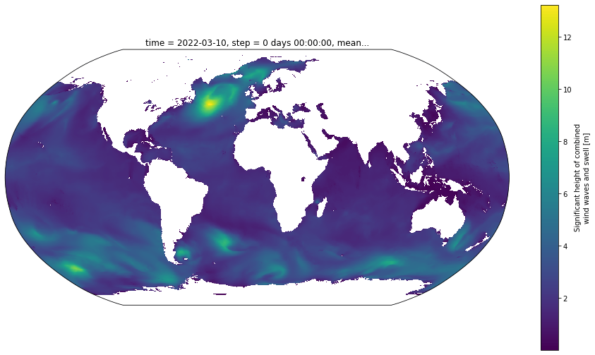
    history:                 2022-03-10T19:02 GRIB to CDM+CF via cfgrib-0.9.1...

We can plot the various data variables, for example the significant height of combined wind waves and swell.

In [5]:

import matplotlib.pyplot as plt
import cartopy.crs as ccrs

projection = ccrs.Robinson()
fig, ax = plt.subplots(figsize=(16, 9), subplot_kw=dict(projection=projection))

ds.swh.plot(ax=ax, transform=ccrs.PlateCarree());

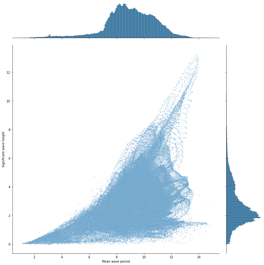
Or the joint distribution between the wave period and height.

In [6]:

import seaborn as sns

grid = sns.jointplot(
    x=ds.mwp.data.ravel(), y=ds.swh.data.ravel(), alpha=0.25, marker=".", height=12
)
grid.ax_joint.set(xlabel="Mean wave period", ylabel="Significant wave height");

GRIB2 files with multiple datasets¶

Some GRIB2 files contain many messages that for separate xarray Datasets. For example, we can find the STAC item containing the atmospheric fields ensemble forecast (stream=enfo) from the ensemble forecast model (type=ef).

In [7]:

search = catalog.search(
    collections=["ecmwf-forecast"],
    query={
        "ecmwf:stream": {"eq": "enfo"},
        "ecmwf:type": {"eq": "ef"},
        "ecmwf:step": {"eq": "0h"},
    },
)
items = search.get_all_items()
print(len(items), "matched")
# select the most recent forecast
item = max(items, key=lambda item: item.datetime)

189 matched

In [8]:

url = item.assets["data"].href
filename, _ = urllib.request.urlretrieve(url)

If we provided just the filename to xarray.open_dataset, we'd get an error from cfgrib saying it can't form a valid DataArray from the file. That's because the GRIB2 file contains multiple data variables that don't form a neat hypercube. Provide filter_by_keys to indicate which subset of the data to read in.

In [9]:

ds = xr.open_dataset(
    filename,
    engine="cfgrib",
    filter_by_keys={"dataType": "pf", "typeOfLevel": "surface"},
)
ds

Now we can plot the skin temperature, skt.

In [ ]:

import matplotlib.pyplot as plt
import cartopy.crs as ccrs

projection = projection = ccrs.Robinson()
fig, ax = plt.subplots(figsize=(16, 9), subplot_kw=dict(projection=projection))

ds.skt[0].plot(ax=ax, transform=ccrs.PlateCarree());

There are many more streams and forecast types available. See the catalog for more.