Accessing GOES data with the Planetary Computer STAC API¶

The Cloud and Moisture Imagery product contains one or more Earth-view images with pixel values identifying brightness values that are scaled to support visual analysis.

Data Access¶

The datasets hosted by the Planetary Computer are available from Azure Blob Storage. We'll use pystac-client to search the Planetary Computer's STAC API for the subset of the data that we care about, and then we'll load the data directly from Azure Blob Storage. We'll specify a modifier so that we can access the data stored in the Planetary Computer's private Blob Storage Containers. See Reading from the STAC API and Using tokens for data access for more.

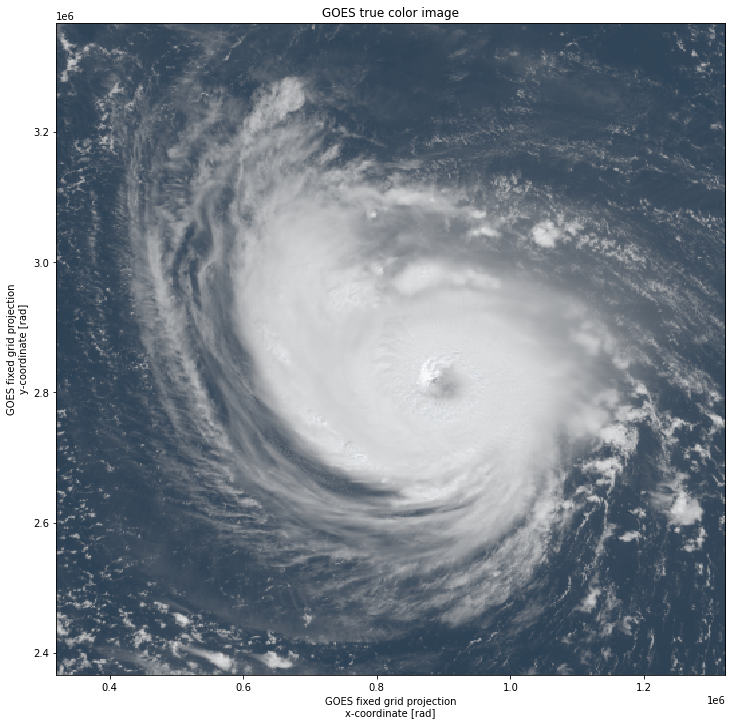
This example will load data from the goes-cmi collection and plot it. We'll select a date and time that captures images of Hurricane Florence.

In [1]:

import pystac_client
import planetary_computer

catalog = pystac_client.Client.open(
    "https://planetarycomputer.microsoft.com/api/stac/v1",
    modifier=planetary_computer.sign_inplace,
)

bbox = [-67.2729, 25.6000, -61.7999, 27.5423]
search = catalog.search(
    collections=["goes-cmi"],
    bbox=bbox,
    datetime=["2018-09-11T13:00:00Z", "2018-09-11T15:40:00Z"],
    limit=1,
    query={"goes:image-type": {"eq": "MESOSCALE"}},
)

item = next(search.items())

The GOES-CMI items have many assets available for the various bands. You can view the full list at https://planetarycomputer.microsoft.com/dataset/goes-cmi. We'll use the blue, red, and near-infrared bands.

In [2]:

import rioxarray
import xarray as xr

bands = ["C01_2km", "C02_2km", "C03_2km"]
common_names = [
    item.assets[band].extra_fields["eo:bands"][0]["common_name"] for band in bands
]
ds = xr.concat(
    [rioxarray.open_rasterio(item.assets[band].href) for band in bands], dim="band"
).assign_coords(band=common_names)
ds

Out[2]:

<xarray.DataArray 'CMI_C01' (band: 3, y: 500, x: 500)>
array([[[ 659,  744,  840, ...,  390,  391,  395],
        [ 602,  742,  817, ...,  390,  391,  392],
        [ 560,  695,  762, ...,  388,  389,  393],
        ...,
        [ 451,  855,  947, ...,  377,  390,  368],
        [ 627, 1028, 1261, ...,  367,  362,  363],
        [1058, 1047, 1400, ...,  367,  362,  391]],

       [[ 444,  522,  634, ...,  117,  117,  116],
        [ 390,  536,  613, ...,  116,  111,  111],
        [ 339,  479,  546, ...,  115,  113,  113],
        ...,
        [ 221,  714,  805, ...,  119,  142,  109],
        [ 425,  911, 1165, ...,  112,  107,  106],
        [ 940,  902, 1321, ...,  111,  105,  136]],

       [[ 393,  480,  593, ...,   54,   52,   53],
        [ 341,  493,  564, ...,   51,   51,   49],
        [ 292,  432,  494, ...,   51,   50,   51],
        ...,
        [ 173,  699,  811, ...,   70,   91,   57],
        [ 412,  916, 1189, ...,   58,   50,   50],
        [ 977,  932, 1385, ...,   57,   49,   87]]], dtype=int16)
Coordinates:
  * band                    (band) <U5 'blue' 'red' 'nir09'
  * x                       (x) float64 3.206e+05 3.226e+05 ... 1.321e+06
  * y                       (y) float64 3.367e+06 3.365e+06 ... 2.367e+06
    goes_imager_projection  int64 0
Attributes:
    add_offset:             0.0
    ancillary_variables:    DQF_C01
    cell_methods:           t: point area: sum (interval: 0.000028 rad)
    coordinates:            band_id_C01 band_wavelength_C01 t y x
    downsampling_method:    average
    long_name:              ABI Cloud and Moisture Imagery reflectance factor
    resolution:             y: 0.000056 rad x: 0.000056 rad
    scale_factor:           0.00031746001332066953
    sensor_band_bit_depth:  10
    standard_name:          toa_lambertian_equivalent_albedo_multiplied_by_co...
    units:                  1
    valid_range:            [   0. 4095.]
    _FillValue:             -1.0
    _Unsigned:              true

GOES doesn't have a true green band, which we need for our true color image. We'll simulate it with a linear combination of the other bands (See Bah et. al (2018) for more on this technique).

In [3]:

green = (
    0.45 * ds.sel(band="red") + 0.1 * ds.sel(band="nir09") + 0.45 * ds.sel(band="blue")
).assign_coords(band="green")
green

Finally, we'll apply a color correction.

In [4]:

import numpy as np

γ = 2.2

rgb = xr.concat([ds, green], dim="band").sel(band=["red", "green", "blue"])
rgb = rgb / rgb.max(dim=["band", "y", "x"])
rgb = np.clip(rgb ** (1 / γ), 0, 1)

In [5]:

import matplotlib.pyplot as plt

fig, ax = plt.subplots(figsize=(12, 12))

rgb.plot.imshow(rgb="band", ax=ax)
ax.set(title="GOES true color image");