Accessing Landsat Collection 2 Level-1 and Level-2 data with the Planetary Computer STAC API¶

The Planetary Computer's Landsat dataset represents a global archive of Level-1 and Level-2 data from from Landsat Collection 2. The dataset is grouped into two STAC Collections:

landsat-c2-l2 for Level-2 data
landsat-c2-l1 for Level-1 data

This notebook demonstrates the use of the Planetary Computer STAC API to query for Landsat data. We will start with an example using Level-2 data and follow with a similar example using Level-1 data.

Environment setup¶

This notebook works with or without an API key, but you will be given more permissive access to the data with an API key.

The Planetary Computer Hub is pre-configured to use your API key.
To use your API key locally, set the environment variable PC_SDK_SUBSCRIPTION_KEY or use pc.settings.set_subscription_key(<YOUR API Key>).

In [1]:

import pystac_client
import planetary_computer
import odc.stac
import matplotlib.pyplot as plt

from pystac.extensions.eo import EOExtension as eo

Data access¶

The datasets hosted by the Planetary Computer are available from Azure Blob Storage. We'll use pystac-client to search the Planetary Computer's STAC API for the subset of the data that we care about, and then we'll load the data directly from Azure Blob Storage. We'll specify a modifier so that we can access the data stored in the Planetary Computer's private Blob Storage Containers. See Reading from the STAC API and Using tokens for data access for more.

In [2]:

catalog = pystac_client.Client.open(
    "https://planetarycomputer.microsoft.com/api/stac/v1",
    modifier=planetary_computer.sign_inplace,
)

Choose an area and time of interest¶

This area is in Redmond, WA, USA, near Microsoft's main campus. We'll search all of 2021, limiting the results to those less than 10% cloudy.

In [3]:

bbox_of_interest = [-122.2751, 47.5469, -121.9613, 47.7458]
time_of_interest = "2021-01-01/2021-12-31"

In [4]:

search = catalog.search(
    collections=["landsat-c2-l2"],
    bbox=bbox_of_interest,
    datetime=time_of_interest,
    query={"eo:cloud_cover": {"lt": 10}},
)

items = search.item_collection()
print(f"Returned {len(items)} Items")

Returned 13 Items

Let's find the least cloudy of the bunch.

In [5]:

selected_item = min(items, key=lambda item: eo.ext(item).cloud_cover)

print(
    f"Choosing {selected_item.id} from {selected_item.datetime.date()}"
    + f" with {selected_item.properties['eo:cloud_cover']}% cloud cover"
)

Choosing LC08_L2SP_046027_20210725_02_T1 from 2021-07-25 with 0.38% cloud cover

Available assets¶

In addition to numerous metadata assets, each Electro-Optical (EO) band is a separate asset.

In [6]:

max_key_length = len(max(selected_item.assets, key=len))
for key, asset in selected_item.assets.items():
    print(f"{key.rjust(max_key_length)}: {asset.title}")

              qa: Surface Temperature Quality Assessment Band
             ang: Angle Coefficients File
             red: Red Band
            blue: Blue Band
            drad: Downwelled Radiance Band
            emis: Emissivity Band
            emsd: Emissivity Standard Deviation Band
            trad: Thermal Radiance Band
            urad: Upwelled Radiance Band
           atran: Atmospheric Transmittance Band
           cdist: Cloud Distance Band
           green: Green Band
           nir08: Near Infrared Band 0.8
          lwir11: Surface Temperature Band
          swir16: Short-wave Infrared Band 1.6
          swir22: Short-wave Infrared Band 2.2
         coastal: Coastal/Aerosol Band
         mtl.txt: Product Metadata File (txt)
         mtl.xml: Product Metadata File (xml)
        mtl.json: Product Metadata File (json)
        qa_pixel: Pixel Quality Assessment Band
       qa_radsat: Radiometric Saturation and Terrain Occlusion Quality Assessment Band
      qa_aerosol: Aerosol Quality Assessment Band
        tilejson: TileJSON with default rendering
rendered_preview: Rendered preview

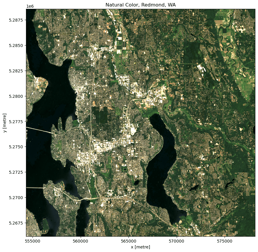
Render a natural color image of the AOI¶

We'll start by loading the red, green, and blue bands for our area of interest into an xarray dataset using odc-stac. We will also load the nir08 band for use in computing an NDVI value in a later example. Note that we pass the sign function from the planetary-computer package so that odc-stac can supply the required Shared Access Signature tokens that are necessary to download the asset data.

In [7]:

bands_of_interest = ["nir08", "red", "green", "blue", "qa_pixel", "lwir11"]
data = odc.stac.stac_load(
    [selected_item], bands=bands_of_interest, bbox=bbox_of_interest
).isel(time=0)
data

Now we'll convert our xarray Dataset to a DataArray and plot the RGB image. We set robust=True in imshow to avoid manual computation of the color limits (vmin and vmax) that is necessary for data not scaled to between 0-1 while also eliminating extreme values that can cause a washed out image.

In [8]:

fig, ax = plt.subplots(figsize=(10, 10))

data[["red", "green", "blue"]].to_array().plot.imshow(robust=True, ax=ax)
ax.set_title("Natural Color, Redmond, WA");

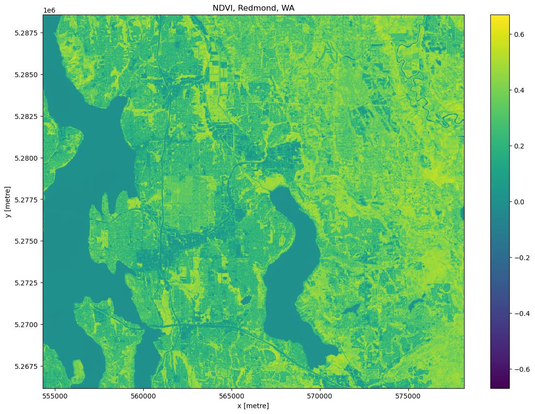
Render an NDVI image of the AOI¶

Landsat has several bands, and with them we can go beyond rendering natural color imagery; for example, the following code computes a Normalized Difference Vegetation Index (NDVI) using the near-infrared and red bands. Note that we convert the red and near infrared bands to a data type that can contain negative values; if this is not done, negative NDVI values will be incorrectly stored.

In [9]:

red = data["red"].astype("float")
nir = data["nir08"].astype("float")
ndvi = (nir - red) / (nir + red)

fig, ax = plt.subplots(figsize=(14, 10))
ndvi.plot.imshow(ax=ax, cmap="viridis")
ax.set_title("NDVI, Redmond, WA");

Selecting specific platforms¶

Landsat Collection 2 Level-2 includes assets from several different Platforms.

In [10]:

catalog.get_collection("landsat-c2-l2").summaries.to_dict()["platform"]

Out[10]:

['landsat-4', 'landsat-5', 'landsat-7', 'landsat-8', 'landsat-9']

You might want to limit your search to a specific platform or platforms, to avoid the Landsat 7 Scan Line Corrector failure, for example. Use the "platform": {"in": ... } query to select specific platforms.

In [11]:

search = catalog.search(
    collections=["landsat-c2-l2"],
    bbox=bbox_of_interest,
    datetime=time_of_interest,
    query={
        "eo:cloud_cover": {"lt": 10},
        "platform": {"in": ["landsat-8", "landsat-9"]},
    },
)
items = search.get_all_items()

Rescaling Temperature Data¶

Landsat Collection 2 Level 2 includes measures of Surface Temperature. We'll look at the surface temperature band TIRS_B10 under the key lwir11. The raw values are rescaled, so you should scale and offset the data before interpreting it. Use the metadata in the asset's raster_bands to find the scale and offset values:

In [12]:

band_info = selected_item.assets["lwir11"].extra_fields["raster:bands"][0]
band_info

Out[12]:

{'unit': 'kelvin',
 'scale': 0.00341802,
 'nodata': 0,
 'offset': 149.0,
 'data_type': 'uint16',
 'spatial_resolution': 30}

To go from the raw values to Kelvin, we apply those values:

In [13]:

temperature = data["lwir11"].astype(float)
temperature *= band_info["scale"]
temperature += band_info["offset"]
temperature[:5, :5]

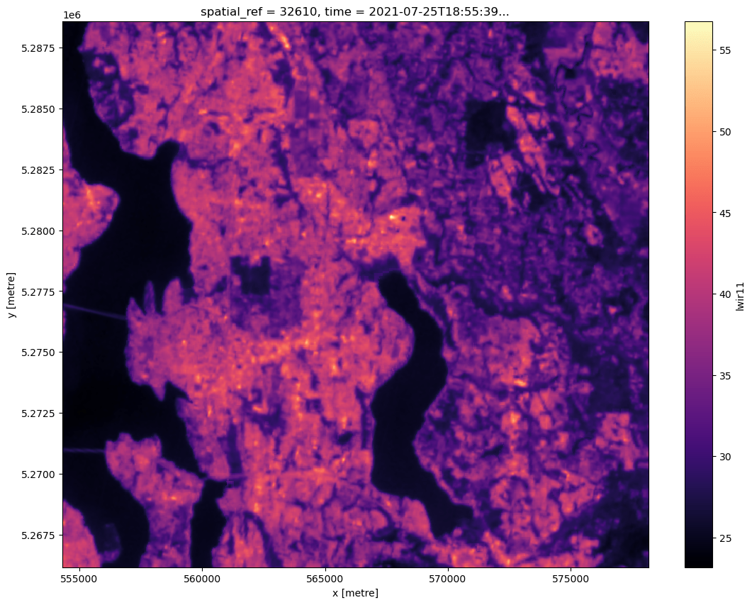
To convert from Kelvin to degrees, subtract 273.15.

In [14]:

celsius = temperature - 273.15
celsius.plot(cmap="magma", size=10);

Landsat Collection 2 Level-1 Data¶

Thus far we have worked with Landsat Collection 2 Level-2 data, which is processed to a consistent set of surface reflectance and surface temperature science products.

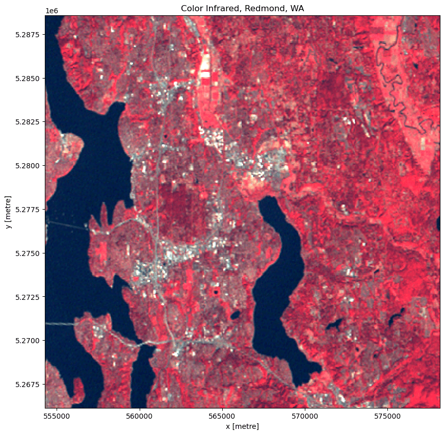
The Planetary Computer also hosts Collection 2 Level-1 data (top of atmosphere values) acquired by the Multispectral Scanner System (MSS) onboard Landsat 1 through 5. These data do not include a blue band, so a natural color image is not possible. We will plot a color infrared image from the nir08, red, and green bands instead.

As before, we use pystac-client to search over the landsat-c2-l1 collection. We'll use the same area of interest and return only those with less than 10% cloud cover.

In [15]:

search = catalog.search(
    collections=["landsat-c2-l1"],
    bbox=bbox_of_interest,
    query={"eo:cloud_cover": {"lt": 10}},
)

items = search.item_collection()
print(f"Returned {len(items)} Items")

Returned 272 Items

Choose the least cloudy Item.

In [16]:

selected_item = min(items, key=lambda item: eo.ext(item).cloud_cover)

print(
    f"Choosing {selected_item.id} from {selected_item.datetime.date()}"
    + f" with {selected_item.properties['eo:cloud_cover']}% cloud cover"
)

Choosing LM05_L1TP_046027_20121004_02_T2 from 2012-10-04 with 0.0% cloud cover

Available assets¶

MSS data has four EO bands assets and a number of metadata files and bands.

In [17]:

max_key_length = len(max(selected_item.assets, key=len))
for key, asset in selected_item.assets.items():
    print(f"{key.rjust(max_key_length)}: {asset.title}")

             red: Red Band
           green: Green Band
           nir08: Near Infrared Band 0.8
           nir09: Near Infrared Band 0.9
         mtl.txt: Product Metadata File (txt)
         mtl.xml: Product Metadata File (xml)
        mtl.json: Product Metadata File (json)
        qa_pixel: Pixel Quality Assessment Band
       qa_radsat: Radiometric Saturation and Dropped Pixel Quality Assessment Band
        tilejson: TileJSON with default rendering
rendered_preview: Rendered preview

We'll use odc-stac to load only the EO bands and area we are interested in.

In [18]:

bands_of_interest = ["nir08", "red", "green"]
data = odc.stac.stac_load(
    [selected_item], bands=bands_of_interest, bbox=bbox_of_interest
).isel(time=0)

cir = data.to_array()

fig, ax = plt.subplots(figsize=(10, 10))
cir.plot.imshow(robust=True, ax=ax)
ax.set_title("Color Infrared, Redmond, WA");