Notebook

Accessing NOAA U.S. Tabular Climate Normals with the Planetary Computer STAC API¶

The NOAA U.S. Tabular Climate Normals provide information about typical climate conditions for thousands of weather station locations across the United States. Normals act both as a ruler to compare current weather and as a predictor of conditions in the near future. The official normals are calculated for a uniform 30 year period, and consist of annual/seasonal, monthly, daily, and hourly averages and statistics of temperature, precipitation, and other climatological variables for each weather station.

This Collection contains tabular weather variable data at weather station locations in GeoParquet format. Data are provided for annual/seasonal, monthly, daily, and hourly frequencies for the following time periods:

30-year Conventional (1991–2020)
30-year Legacy (1981–2010)
15-year Supplemental (2006–2020)

Documentation for this dataset is available at the Planetary Computer Data Catalog.

Data Access¶

This notebook works with or without an API key, but you will be given more permissive access to the data with an API key. The Planetary Computer Hub sets the environment variable "PC_SDK_SUBSCRIPTION_KEY" when your server is started. The API key may be manually set via the following code:

pc.settings.set_subscription_key(<YOUR API Key>)

The datasets hosted by the Planetary Computer are available from Azure Blob Storage. We'll use pystac-client to search the Planetary Computer's STAC API for the subset of the data that we care about, and then we'll load the data directly from Azure Blob Storage. We'll specify a modifier so that we can access the data stored in the Planetary Computer's private Blob Storage Containers. See Reading from the STAC API and Using tokens for data access for more.

In [1]:

import planetary_computer
import pystac_client

# Open the Planetary Computer STAC API
catalog = pystac_client.Client.open(
    "https://planetarycomputer.microsoft.com/api/stac/v1",
    modifier=planetary_computer.sign_inplace,
)

collection = catalog.get_collection("noaa-climate-normals-tabular")

In [2]:

# Get Items
items = list(collection.get_all_items())
items

Out[2]:

[<Item id=2006_2020-monthly>,
 <Item id=2006_2020-hourly>,
 <Item id=2006_2020-daily>,
 <Item id=2006_2020-annualseasonal>,
 <Item id=1991_2020-monthly>,
 <Item id=1991_2020-hourly>,
 <Item id=1991_2020-daily>,
 <Item id=1991_2020-annualseasonal>,
 <Item id=1981_2010-monthly>,
 <Item id=1981_2010-hourly>,
 <Item id=1981_2010-daily>,
 <Item id=1981_2010-annualseasonal>]

Available Assets & Metadata¶

Let's display the available assets and metadata for the NOAA U.S. Tabular Climate Normals product.

In [3]:

import rich.table

# Assets
t_assets = rich.table.Table("Key", "Value")
for key, asset in items[0].assets.items():
    t_assets.add_row(key, asset.title)
t_assets

Out[3]:

┏━━━━━━━━━━━━┳━━━━━━━━━━━━━━┓
┃ Key        ┃ Value        ┃
┡━━━━━━━━━━━━╇━━━━━━━━━━━━━━┩
│ geoparquet │ Dataset root │
└────────────┴──────────────┘

In [4]:

# Metadata
t_metadata = rich.table.Table("Key", "Value")
for k, v in sorted(items[0].properties.items()):
    if k != "table:columns":
        t_metadata.add_row(k, str(v))
t_metadata

Out[4]:

┏━━━━━━━━━━━━━━━━━━━━━━━━━━━━━━━━┳━━━━━━━━━━━━━━━━━━━━━━━━━━━━━━━━━━━━━━━━━━━━━━━━━━━━━━━━━━━━━━━━━━━━━━━━━━━━━━━━┓
┃ Key                            ┃ Value                                                                          ┃
┡━━━━━━━━━━━━━━━━━━━━━━━━━━━━━━━━╇━━━━━━━━━━━━━━━━━━━━━━━━━━━━━━━━━━━━━━━━━━━━━━━━━━━━━━━━━━━━━━━━━━━━━━━━━━━━━━━━┩
│ created                        │ 2023-01-13T17:12:43.569562Z                                                    │
│ datetime                       │ None                                                                           │
│ end_datetime                   │ 2020-12-31T23:59:59Z                                                           │
│ noaa_climate_normals:frequency │ monthly                                                                        │
│ noaa_climate_normals:period    │ 2006-2020                                                                      │
│ proj:epsg                      │ 4269                                                                           │
│ sci:publications               │ [{'doi': '10.1175/BAMS-D-11-00197.1', 'citation': "Arguez, A., I. Durre, S.    │
│                                │ Applequist, R. Vose, M. Squires, X. Yin, R. Heim, and T. Owen, 2012: NOAA's    │
│                                │ 1981-2010 climate normals: An overview. Bull. Amer. Meteor. Soc., 93,          │
│                                │ 1687-1697. DOI: 10.1175/BAMS-D-11-00197.1."}]                                  │
│ start_datetime                 │ 2006-01-01T00:00:00Z                                                           │
│ table:row_count                │ 161652                                                                         │
│ title                          │ Monthly Climate Normals for Period 2006-2020                                   │
└────────────────────────────────┴────────────────────────────────────────────────────────────────────────────────┘

Loading the GeoParquet dataset¶

Now let's load a STAC item into a tabular format.

In [5]:

import geopandas

df = geopandas.read_parquet(
    asset.href,
    storage_options=asset.extra_fields["table:storage_options"],
    columns=["STATION", "month", "MLY-PRCP-NORMAL", "geometry"],
)

Displaying the tabular data¶

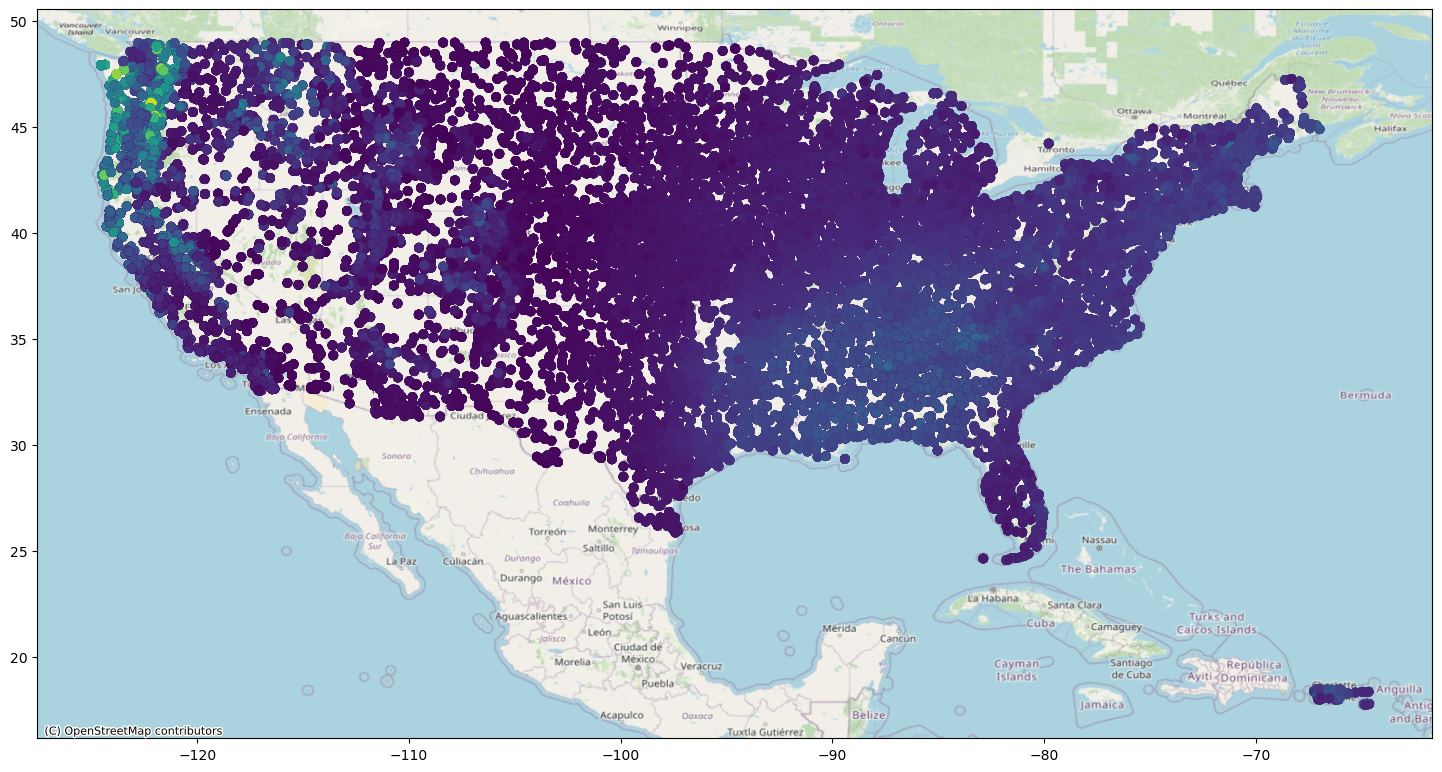
Let's display the NOAA U.S. Tabular Climate Normals for the Continental United States and Puerto Rico.

In [6]:

import contextily

ax = df.cx[-125:24, -65:50.5].plot(figsize=(18, 18), column="MLY-PRCP-NORMAL")
contextily.add_basemap(
    ax, crs=df.crs.to_string(), source=contextily.providers.OpenStreetMap.Mapnik
)