Notebook

Accessing Sentinel-1 Level-1 GRD data with the Planetary Computer STAC API¶

The Level-1 Ground Range Detected (GRD) products in this Collection consist of focused SAR data that has been detected, multi-looked and projected to ground range using the Earth ellipsoid model WGS84.

Environment setup¶

This notebook works with or without an API key, but you will be given more permissive access to the data with an API key.

The Planetary Computer Hub is pre-configured to use your API key.
To use your API key locally, set the environment variable PC_SDK_SUBSCRIPTION_KEY or use planetary_computer.settings.set_subscription_key(<YOUR API Key>)

In [1]:

import pystac_client
import planetary_computer
import rioxarray
import xarray as xr
import numpy as np
import rich.table

Data access¶

The datasets hosted by the Planetary Computer are available from Azure Blob Storage. We'll use pystac-client to search the Planetary Computer's STAC API for the subset of the data that we care about, and then we'll load the data directly from Azure Blob Storage. We'll specify a modifier so that we can access the data stored in the Planetary Computer's private Blob Storage Containers. See Reading from the STAC API and Using tokens for data access for more.

In [2]:

catalog = pystac_client.Client.open(
    "https://planetarycomputer.microsoft.com/api/stac/v1",
    modifier=planetary_computer.sign_inplace,
)

Choose an area and time of interest¶

We'll query for images over Microsoft's main campus in Redmond, Washington during January 2021.

In [3]:

bbox_of_interest = [-122.2751, 47.5469, -121.9613, 47.7458]
time_of_interest = "2021-01-01/2021-12-31"

search = catalog.search(
    collections=["sentinel-1-grd"],
    bbox=bbox_of_interest,
    datetime=time_of_interest,
)

items = search.item_collection()
print(f"Returned {len(items)} Items")

Returned 115 Items

We can use the rendered_preview asset to get a quick preview of the item. This uses the Planetary Computer's data API to dynamically render an image from the underlying assets.

In [4]:

from IPython.display import Image

item = items[0]
Image(url=item.assets["rendered_preview"].href)

Out[4]:

Inspect the STAC metadata¶

The STAC metadata includes information about when and how the assets were acquired, including metadata from the SAR and Satellite extensions.

In [5]:

table = rich.table.Table("key", "value")
for k, v in sorted(item.properties.items()):
    table.add_row(k, str(v))

table

Out[5]:

┏━━━━━━━━━━━━━━━━━━━━━━━━━━━━━━━━━━━━━━━┳━━━━━━━━━━━━━━━━━━━━━━━━━━━━━━━━━━┓
┃ key                                   ┃ value                            ┃
┡━━━━━━━━━━━━━━━━━━━━━━━━━━━━━━━━━━━━━━━╇━━━━━━━━━━━━━━━━━━━━━━━━━━━━━━━━━━┩
│ constellation                         │ Sentinel-1                       │
│ datetime                              │ 2021-12-22T14:21:07.534562Z      │
│ end_datetime                          │ 2021-12-22 14:21:20.033489+00:00 │
│ platform                              │ SENTINEL-1B                      │
│ s1:datatake_id                        │ 235856                           │
│ s1:instrument_configuration_ID        │ 2                                │
│ s1:orbit_source                       │ RESORB                           │
│ s1:processing_level                   │ 1                                │
│ s1:product_timeliness                 │ Fast-24h                         │
│ s1:resolution                         │ high                             │
│ s1:shape                              │ [25981, 16680]                   │
│ s1:slice_number                       │ 9                                │
│ s1:total_slices                       │ 16                               │
│ sar:center_frequency                  │ 5.405                            │
│ sar:frequency_band                    │ C                                │
│ sar:instrument_mode                   │ IW                               │
│ sar:looks_azimuth                     │ 1                                │
│ sar:looks_equivalent_number           │ 4.4                              │
│ sar:looks_range                       │ 5                                │
│ sar:observation_direction             │ right                            │
│ sar:pixel_spacing_azimuth             │ 10                               │
│ sar:pixel_spacing_range               │ 10                               │
│ sar:polarizations                     │ ['VV', 'VH']                     │
│ sar:product_type                      │ GRD                              │
│ sar:resolution_azimuth                │ 22                               │
│ sar:resolution_range                  │ 20                               │
│ sat:absolute_orbit                    │ 30139                            │
│ sat:orbit_state                       │ descending                       │
│ sat:platform_international_designator │ 2016-025A                        │
│ sat:relative_orbit                    │ 13                               │
│ start_datetime                        │ 2021-12-22 14:20:55.035634+00:00 │
└───────────────────────────────────────┴──────────────────────────────────┘

The item's data assets will be some combination of vh, vv, hv, and hh, depending on the polarization the signal was transmitted and received in. In this case, the item has vv and vh assets. In general, check the sar:polarizations field for what is available.

In [6]:

item.properties["sar:polarizations"]

Out[6]:

['VV', 'VH']

Visualize the assets¶

Next, we'll use rioxarray to load the data. Since we're just vizualizing the data we'll load one of the lower-resolution overviews.

In [7]:

vv = (
    rioxarray.open_rasterio(item.assets["vv"].href, overview_level=2)
    .astype(float)
    .squeeze()
)
vh = (
    rioxarray.open_rasterio(item.assets["vh"].href, overview_level=2)
    .astype(float)
    .squeeze()
)

We can plot this distribution of the pixel values, to get a sense for their range. The raw values are fairly skewed, so it's common to render with an amplitude scale (taking the square root of the value) or a dB scale ($10 \times log_{10}$ of the value).

In [8]:

import pandas as pd
import seaborn as sns

raw = vv.where(lambda x: x > 0).data.ravel()
df = (
    pd.DataFrame({"power": raw, "amplitude": np.sqrt(raw), "dB": 10 * np.log10(raw)})
    .dropna()
    .melt(value_vars=["power", "amplitude", "dB"], var_name="kind")
)

In [9]:

g = sns.FacetGrid(df, sharex=False, col="kind")
g.map(sns.histplot, "value", bins=30);

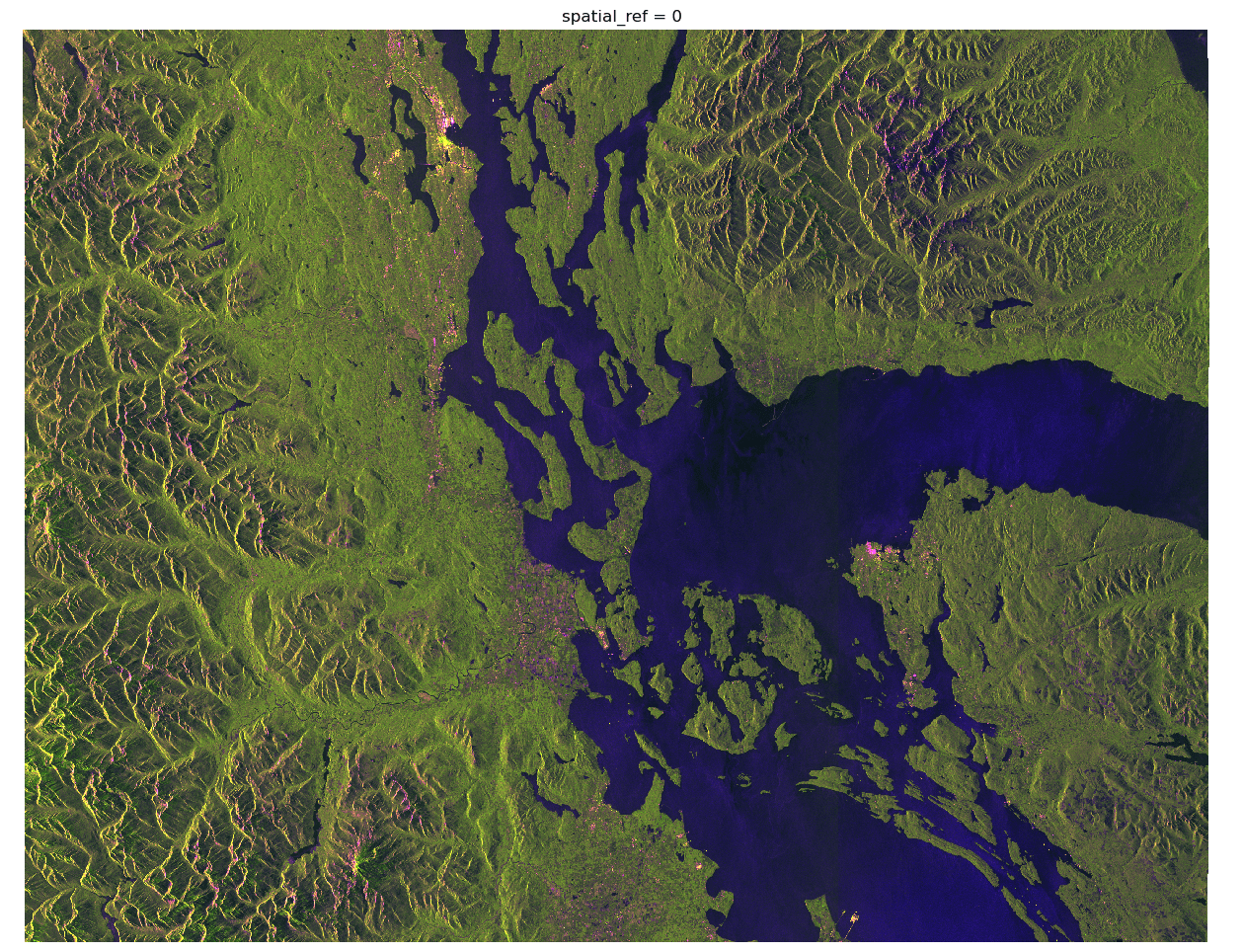
Now let's recreate the false-color image from the data API, using a combination of the two bands. We'll use vv as the red band, vh as the green band, and vv / vh as the green band. We'll rescale it as well (using values from the mosaic/info endpoint).

In [10]:

r = vv / 600
g = vh / 270
b = (vv / vh) / 9
data = xr.concat([r, g, b], dim="band").clip(0, 1).where(lambda x: x > 0)
img = data.plot.imshow(rgb="band", size=12)
img.axes.set_axis_off()

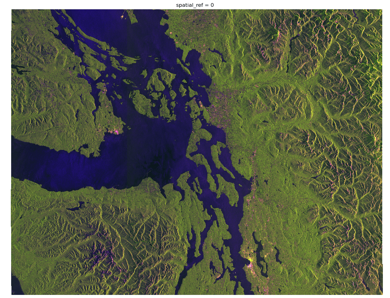
By default, some Sentinel-1 GRD images may appear "upside-down". Seattle, the brightest spot area, appears towards the top-left of the image, despite being in the southwest of the area.

Whether the data needs to be flipped depends on the mode the satellite was in when the image was captured, which is available from the sat:orbit_state property in the STAC metadata.

In [11]:

item.properties["sat:orbit_state"]

Out[11]:

'descending'

In this case, the satellite was in "descending" mode, and so we need to flip the image if we north to be up.

In [12]:

img = np.flip(data, axis=(1, 2)).clip(0, 1).plot.imshow(size=12)
img.axes.set_axis_off()

GRD Products¶

The resolution and bands available depend on the acquisition mode and level of multi-looking.

Stripmap (SM)
Interferometric Wide Swath (IW)
Extra-Wide swath (EW)
Wave (WV)

From the Sentinel-1 User Guide:

The primary conflict-free modes are IW, with VV+VH polarisation over land, and WV, with VV polarisation, over open ocean. EW mode is primarily used for wide area coastal monitoring including ship traffic, oil spill and sea-ice monitoring. SM mode is only used for small islands and on request for extraordinary events such as emergency management.

You can query for specific modes using the sar:instrument_mode property.

In [13]:

search = catalog.search(
    collections=["sentinel-1-grd"],
    query={
        "sar:instrument_mode": {"eq": "SM"},
        "sar:polarizations": {"eq": ["VV", "VH"]},
    },
    limit=5,
)

gen = search.items()
item = next(gen)

Image(url=item.assets["rendered_preview"].href)

Out[13]:

Terrain Correction¶

Those wishing to use a terrain corrected Sentinel-1 product can use the pre-computed Sentinel-1 RTC collection from the Planetary Computer, or apply their own customizable terrain correction.