Adjusting for the Sentinel-2 Baseline Change
On January 25th, 2022 the European Space Agency implemented a change to the processing baseline for Sentinel-2 data that affects both L1C and the L2A data hosted by the Planetary Computer.
The crux of the change is an offset to the L1C image reflectance data, which propagates to the L2A data hosted by the Planetary Computer.
As explained by ESA:
This evolution allows avoiding the loss of information due to clamping of negative values in the predefined range
[1-32767]occurring over dark surfaces.
The presence of this offset in newer data makes it inappropriate to (naively) compare data from before and after the baseline change. Trying to apply a machine learning model trained on the old baseline to (unadjusted) imagery from the new baseline will yield incorrect results. And trying to train a machine learning model on old and (unadjusted) new data will likely result in much worse performance.
This notebook demonstrates how the change affects the Sentinel-2 L2A data hosted on the Planetary Computer and how to harmonize the new data to be comparable to the old data.
import pystac_client
import planetary_computer
import xarray as xr
import matplotlib.pyplot as plt
import skimage.exposure
import seaborn as sns
import stackstac
import datetime
The harmonize_to_old function harmonizes new (post January 25th, 2022) Sentinel 2 data to be comparable to older data. It expects an xarray DataArray similar to those returned by stackstac.
def harmonize_to_old(data):
    """
    Harmonize new Sentinel-2 data to the old baseline.

    Parameters
    ----------
    data: xarray.DataArray
        A DataArray with four dimensions: time, band, y, x

    Returns
    -------
    harmonized: xarray.DataArray
        A DataArray with all values harmonized to the old
        processing baseline.
    """
    cutoff = datetime.datetime(2022, 1, 25)
    offset = 1000
    bands = [
        "B01",
        "B02",
        "B03",
        "B04",
        "B05",
        "B06",
        "B07",
        "B08",
        "B8A",
        "B09",
        "B10",
        "B11",
        "B12",
    ]

    old = data.sel(time=slice(cutoff))

    to_process = list(set(bands) & set(data.band.data.tolist()))
    new = data.sel(time=slice(cutoff, None)).drop_sel(band=to_process)

    new_harmonized = data.sel(time=slice(cutoff, None), band=to_process).clip(offset)
    new_harmonized -= offset

    new = xr.concat([new, new_harmonized], "band").sel(band=data.band.data.tolist())
    return xr.concat([old, new], dim="time")
To demonstrate the problem, we'll load an "old" scene with the old processing baseline of 03.00, and a "new" scene with a new processing baseline of 04.00.
s2 = pystac_client.Client.open(
    "https://planetarycomputer.microsoft.com/api/stac/v1/",
    modifier=planetary_computer.sign_inplace,
).get_collection("sentinel-2-l2a")

old = s2.get_item("S2B_MSIL2A_20220106T021339_R060_T50KPC_20220107T033435")
new = s2.get_item("S2A_MSIL2A_20230116T021341_R060_T50KPC_20230116T112621")
We'll stack these together, cropping out a small section of the image to speed up loading.
bounds = (600000, 7690240, 610000, 7700240)
assets = ["B02", "B03", "B04", "B05", "B06", "AOT"]
ds = stackstac.stack([old, new], assets=assets, bounds=bounds)
ds
<xarray.DataArray 'stackstac-7f8b9fd36f84dee2d0c759174b259b65' (time: 2,
                                                                band: 6,
                                                                y: 1000, x: 1000)>
dask.array<fetch_raster_window, shape=(2, 6, 1000, 1000), dtype=float64, chunksize=(1, 1, 1000, 1000), chunktype=numpy.ndarray>
Coordinates: (12/44)
  * time                                     (time) datetime64[ns] 2022-01-06...
    id                                       (time) <U54 'S2B_MSIL2A_20220106...
  * band                                     (band) <U3 'B02' 'B03' ... 'AOT'
  * x                                        (x) float64 6e+05 6e+05 ... 6.1e+05
  * y                                        (y) float64 7.7e+06 ... 7.69e+06
    s2:reflectance_conversion_factor         (time) float64 1.034 1.034
    ...                                       ...
    proj:bbox                                object {600000.0, 7690240.0, 780...
    gsd                                      (band) float64 10.0 10.0 ... 10.0
    common_name                              (band) object 'blue' ... None
    center_wavelength                        (band) object 0.49 0.56 ... None
    full_width_half_max                      (band) object 0.098 0.045 ... None
    epsg                                     int64 32750
Attributes:
    spec:        RasterSpec(epsg=32750, bounds=(600000.0, 7690240.0, 610000.0...
    crs:         epsg:32750
    transform:   | 10.00, 0.00, 600000.00|\n| 0.00,-10.00, 7700240.00|\n| 0.0...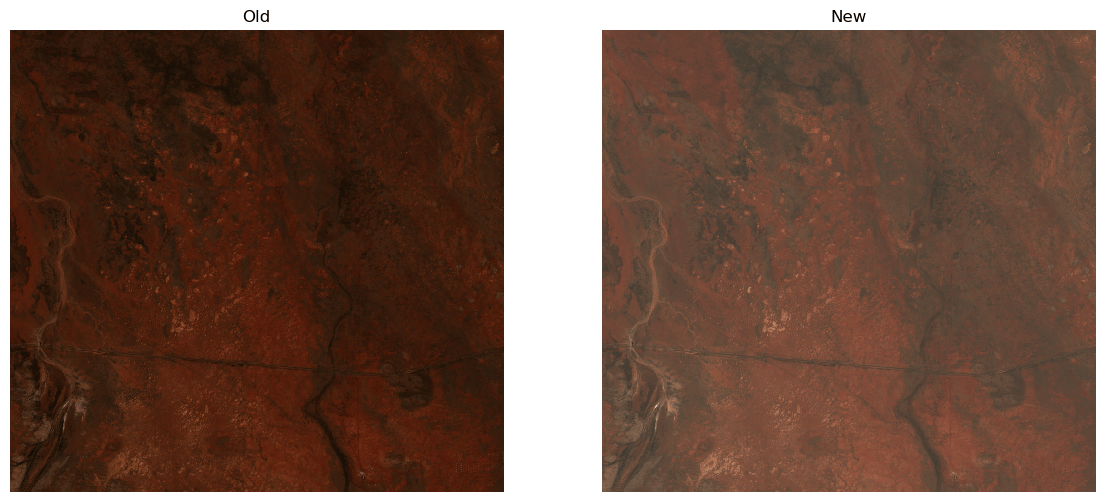
resolution: 10.0If we plot the red, green, and blue bands of the two datetimes, we'll see that the "old" data looks relatively dark compared to the "new" data.
fig, axes = plt.subplots(ncols=2, figsize=(14, 6))

img = ds.sel(band=["B04", "B03", "B02"]).compute()
img = xr.apply_ufunc(skimage.exposure.rescale_intensity, img)

img.isel(time=0).plot.imshow(rgb="band", ax=axes[0])
axes[0].set(title="Old")

img.isel(time=1).plot.imshow(rgb="band", ax=axes[1])
axes[1].set(title="New")
for ax in axes:
    ax.set_axis_off()
By taking the histogram of, say, the green band, we'll see that the new data are shifted to the right.
fig, ax = plt.subplots(figsize=(12, 8))

hist, bins = skimage.exposure.histogram(ds.isel(time=0, band=1).data.compute())
ax.plot(bins, hist, label="Old")

hist, bins = skimage.exposure.histogram(ds.isel(time=1, band=1).data.compute())
ax.plot(bins, hist, label="New")
plt.legend()
sns.despine()

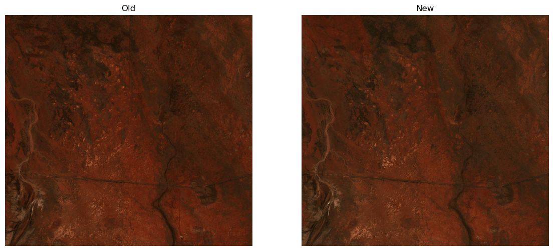
Now, let's harmonize data, shifting the new data to make it comparable to the old.
harmonized = harmonize_to_old(ds)
Now the RGB images look much more similar:
fig, axes = plt.subplots(ncols=2, figsize=(14, 6))

img = harmonized.sel(band=["B04", "B03", "B02"]).compute()
img = xr.apply_ufunc(skimage.exposure.rescale_intensity, img)

img.isel(time=0).plot.imshow(rgb="band", ax=axes[0])
axes[0].set(title="Old")

img.isel(time=1).plot.imshow(rgb="band", ax=axes[1])
axes[1].set(title="New")
for ax in axes:
    ax.set_axis_off()
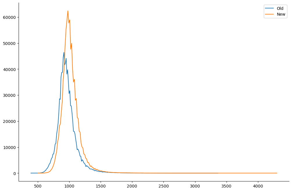
And the histograms now mostly overlap. Any remaining differences are a result of the two scenes being captured a year apart.
fig, ax = plt.subplots(figsize=(12, 8))

hist, bins = skimage.exposure.histogram(harmonized.isel(time=0, band=1).data.compute())
ax.plot(bins, hist, label="Old")

hist, bins = skimage.exposure.histogram(harmonized.isel(time=1, band=1).data.compute())
ax.plot(bins, hist, label="New")
plt.legend()
sns.despine()