United States 2020 Census data
In this tutorial, you will explore various subsets of geographic data in the United States 2020 Census. You will learn how the data is structured and how to access the data.
The data consists of two groups:
- Census data by census block boundaries: This group contains data for each census block, grouped by US counties. Census blocks are the smallest available unit made available by the US Census Bureau. This group also includes population totals broken down by census block, available in a second table.
- Census data by cartographic boundaries: This group contains data that is aggregated by 29 different geographic boundaries, ranging from block groups to regional datasets such as metropolitan divisions and states. This group does not include any demographic information.
This notebook contains details about all geographic datasets within the 2020 census data. Use the table of contents to jump to any section relevant to you. For a brief introduction, Accessing US Census data with the Planetary Computer STAC API.
Table of Contents
- Accessing the Data
- Import Dependencies
- Census data by census block boundaries
- Census Block Boundaries (8,180,866 features)
- Census data by cartographic boundaries
- American Indian Area Geographies
- American Indian/Alaska Native Areas/Hawaiian Home Lands (704 features)
- American Indian Tribal Subdivisions (484 features)
- Alaska Native Regional Corporations (12 features)
- Tribal Block Groups (934 features)
- Tribal Census Tracts (492 features)
- Census Block Groups (242,305 features)
- Census Tracts (85,190 features)
- Congressional Districts (441 features)
- Consolidated Cities (8 features)
- Counties (3,234 features)
- Counties within Congressional Districts (3,836 features)
- County Subdivisions (36,502 features)
- Divisions (9 features)
- Metropolitan and Micropolitan Statistical Areas and Related Statistical Areas
- Core Based Statistical Areas (939 features)
- Combined Statistical Areas (175 features)
- Metropolitan Divisions (31 features)
- New England City and Town Areas (40 features)
- New England City and Town Areas Division (11 features)
- Combined New England City and Town Areas (7 features)
- Places (32,188 features)
- Regions (4 features)
- School Districts
- Elementary (1,945 features)
- Secondary (473 features)
- Unified (10,867 features)
- State Legislative Districts
- Lower Chamber (4,829 features)
- Upper Chamber (1,958 features)
- States (56 features)
- Subbarrios (145 features)
- United States Outline (1 feature)
- Voting Districts (158,320 features)
- American Indian Area Geographies
Accessing the Data
Like other datasets on the Planetary Computer, US Census datasets are cataloged using STAC. Each table, corresponding a particular level of cartographic aggregation, is available as a STAC item under the us-census collection.
import pystac_client
import planetary_computer

catalog = pystac_client.Client.open(
    "https://planetarycomputer.microsoft.com/api/stac/v1/",
    modifier=planetary_computer.sign_inplace,
)
census = catalog.get_collection("us-census")
census
- type "Collection"
- id "us-census"
- stac_version "1.0.0"
- description "The [2020 Census](https://www.census.gov/programs-surveys/decennial-census/decade/2020/2020-census-main.html) counted every person living in the United States and the five U.S. territories. It marked the 24th census in U.S. history and the first time that households were invited to respond to the census online. The tables included on the Planetary Computer provide information on population and geographic boundaries at various levels of cartographic aggregation. "
links [] 6 items
0
- rel "items"
- href "https://planetarycomputer.microsoft.com/api/stac/v1/collections/us-census/items"
- type "application/geo+json"
1
- rel "parent"
- href "https://planetarycomputer.microsoft.com/api/stac/v1/"
- type "application/json"
2
- rel "root"
- href "https://planetarycomputer.microsoft.com/api/stac/v1/"
- type "application/json"
- title "Microsoft Planetary Computer STAC API"
3
- rel "self"
- href "https://planetarycomputer.microsoft.com/api/stac/v1/collections/us-census"
- type "application/json"
4
- rel "license"
- href "https://www.census.gov/about/policies/open-gov/open-data.html"
- type "text/html"
- title "U.S. Census Open Data Policy"
5
- rel "describedby"
- href "https://planetarycomputer.microsoft.com/dataset/us-census"
- type "text/html"
- title "Human readable dataset overview and reference"
stac_extensions [] 2 items
- 0 "https://stac-extensions.github.io/item-assets/v1.0.0/schema.json"
- 1 "https://stac-extensions.github.io/table/v1.2.0/schema.json"
item_assets
data
- type "application/x-parquet"
roles [] 1 items
- 0 "data"
- title "Dataset root"
table:storage_options
- account_name "ai4edataeuwest"
table:tables [] 30 items
0
- name "American Indian/Alaska Native Areas/Hawaiian Home Lands (AIANNH)"
- description "This file contains data for legal and statistical [American Indian/Alaska Native Areas/Hawaiian Home Lands (AIANNH)](https://www.census.gov/programs-surveys/geography/about/glossary.html#par_textimage_1) entities published by the US Census Bureau."
- msft:item_name "cb_2020_us_aiannh_500k"
1
- name "American Indian Tribal Subdivisions (AITSN)"
- description "This file contains data on [American Indian Tribal Subdivisions](https://www.census.gov/programs-surveys/geography/about/glossary.html#par_textimage_1). These areas are the legally defined subdivisions of American Indian Reservations (AIR), Oklahoma Tribal Statistical Areas (OTSA), and Off-Reservation Trust Land (ORTL)."
- msft:item_name "cb_2020_us_aitsn_500k"
2
- name "Alaska Native Regional Corporations (ANRC)"
- description "This file contains data on [Alaska Native Regional Corporations](https://www.census.gov/programs-surveys/geography/about/glossary.html#par_textimage_1), which are corporations created according to the Alaska Native Claims Settlement Act. "
- msft:item_name "cb_2020_02_anrc_500k"
3
- name "Tribal Block Groups (TBG)"
- description "This file includes data on [Tribal Block Groups](https://www.census.gov/programs-surveys/geography/about/glossary.html#par_textimage_26), which are subdivisions of Tribal Census Tracts. These block groups can extend over multiple AIRs and ORTLs due to areas not meeting Block Group minimum population thresholds."
- msft:item_name "cb_2020_us_tbg_500k"
4
- name "Tribal Census Tracts (TTRACT)"
- description "This file includes data on [Tribal Census Tracts](https://www.census.gov/programs-surveys/geography/about/glossary.html#par_textimage_27) which are relatively small statistical subdivisions of AIRs and ORTLs defined by federally recognized tribal government officials in partnership with the Census Bureau. Due to population thresholds, the Tracts may consist of multiple non-contiguous areas."
- msft:item_name "cb_2020_us_ttract_500k"
5
- name "Census Block Groups (BG)"
- description "This file contains data on [Census Block Groups](https://www.census.gov/programs-surveys/geography/about/glossary.html#par_textimage_4). These groups are the second smallest geographic grouping. They consist of clusters of blocks within the same census tract that share the same first digit of their 4-character census block number. Census Block Groups generally contain between 600 and 3,000 people and generally cover contiguous areas."
- msft:item_name "cb_2020_us_bg_500k"
6
- name "Census Tracts (TRACT)"
- description "This file contains data on [Census Tracts](https://www.census.gov/programs-surveys/geography/about/glossary.html#par_textimage_13) which are small and relatively permanent statistical subdivisions of a county or equivalent entity. Tract population size is generally between 1,200 and 8,000 people with an ideal size of 4,000. Boundaries tend to follow visible and identifiable features and are usually contiguous areas."
- msft:item_name "cb_2020_us_tract_500k"
7
- name "Congressional Districts: 116th Congress (CD116)"
- description "This file contains data on the [Congressional Districts](https://www.census.gov/programs-surveys/geography/about/glossary.html#par_textimage_9) for the 116th Congress. "
- msft:item_name "cb_2020_us_cd116_500k"
8
- name "Consolidated Cities (CONCITY)"
- description "This file contains data on [Consolidated Cities](https://www.census.gov/programs-surveys/geography/about/glossary.html#par_textimage_8). These are areas where one or several other incorporated places in a county or Minor Civil Division are included in a consolidated government but still exist as separate legal entities."
- msft:item_name "cb_2020_us_concity_500k"
9
- name "Counties (COUNTY)"
- description "This file contains data on [Counties and Equivalent Entities](https://www.census.gov/programs-surveys/geography/about/glossary.html#par_textimage_12). These are the primary legal divisions of states. Most states use the term "counties," but other terms such as "Parishes," "Municipios," or "Independent Cities" may be used. "
- msft:item_name "cb_2020_us_county_500k"
10
- name "Counties within Congressional Districts: 116th Congress (COUNTY_within_CD116)"
- description "This file contains data on Counties within Congressional Districts."
- msft:item_name "cb_2020_us_county_within_cd116_500k"
11
- name "County Subdivisions (COUSUB)"
- description "This file contains [County Subdivisions](https://www.census.gov/programs-surveys/geography/about/glossary.html#par_textimage_11), which are the primary divisions of counties and equivalent entities. These divisions vary from state to state and include Barrios, Purchases, Townships, and other types of legal and statistical entities. "
- msft:item_name "cb_2020_us_cousub_500k"
12
- name "Divisions (DIVISION)"
- description "This file contains data on [Divisions](https://www.census.gov/programs-surveys/geography/about/glossary.html#par_textimage_10) of the US. This file is similar to the Regions file but contains more divisions and encompasses several states per division."
- msft:item_name "cb_2020_us_division_500k"
13
- name "Core Based Statistical Areas (CBSAs)"
- description "This file contains data on [Core Based Statistical Areas (CBSAs)](https://www.census.gov/programs-surveys/geography/about/glossary.html#par_textimage_7). This encompasses all metropolitan and micropolitan statistical areas."
- msft:item_name "cb_2020_us_cbsa_500k"
14
- name "Combined Statistical Areas (CSA)"
- description "This file contains data on [Combined Statistical Areas](https://www.census.gov/programs-surveys/geography/about/glossary.html#par_textimage_7), which are areas that consist of two or more adjacent CBSAs that have significant employment interchanges."
- msft:item_name "cb_2020_us_csa_500k"
15
- name "Metropolitan Divisions (METDIV)"
- description "This file contains data on [Metropolitan Divisions](https://www.census.gov/programs-surveys/geography/about/glossary.html#par_textimage_7). These areas are groupings of counties or equivalent entities within a metropolitan statistical area with a core of 2.5 million inhabitants and one or more main counties that represent employment centers, plus adjacent counties with commuting ties."
- msft:item_name "cb_2020_us_metdiv_500k"
16
- name "New England City and Town Areas (NECTA)"
- description "This file contains [New England City and Town Areas](https://www.census.gov/programs-surveys/geography/about/glossary.html#par_textimage_7), which encompass metropolitan and micropolitan statistical areas and urban clusters in New England."
- msft:item_name "cb_2020_us_necta_500k"
17
- name "New England City and Town Area Division (NECTADIV)"
- description "This file contains [New England City and Town Areas Divisions](https://www.census.gov/programs-surveys/geography/about/glossary.html#par_textimage_7), which are smaller groupings of cities and towns in New England that contain a single core of 2.5 million inhabitants. Each division must have a total population of 100,000 or more."
- msft:item_name "cb_2020_us_nectadiv_500k"
18
- name "Combined New England City and Town Areas (CNECTA)"
- description "This file contains data on [Combined New England City and Town Areas](https://www.census.gov/programs-surveys/geography/about/glossary.html#par_textimage_7), consisting of two or more adjacent NECTAs that have significant employment interchanges."
- msft:item_name "cb_2020_us_cnecta_500k"
19
- name "Places (PLACE)"
- description "This file contains [Places](https://www.census.gov/programs-surveys/geography/about/glossary.html#par_textimage_14) which are Incorporated Places (legal entities) and Census Designated Places (CDPs, statistical entities). An incorporated place usually is a city, town, village, or borough but can have other legal descriptions. CDPs are settled concentrations of population that are identifiable by name but are not legally incorporated."
- msft:item_name "cb_2020_us_place_500k"
20
- name "Regions (REGION)"
- description "This file contains [Regions](https://www.census.gov/programs-surveys/geography/about/glossary.html#par_textimage_10) of the US and encompasses several states per division."
- msft:item_name "cb_2020_us_region_500k"
21
- name "School Districts - Elementary (ELSD)"
- description "This file contains [Elementary School Districts](https://www.census.gov/programs-surveys/geography/about/glossary.html#par_textimage_23), referring to districts with elementary schools."
- msft:item_name "cb_2020_us_elsd_500k"
22
- name "School Districts - Secondary (SCSD)"
- description "This file contains [Secondary School Districts](https://www.census.gov/programs-surveys/geography/about/glossary.html#par_textimage_23), referring to districts with secondary schools."
- msft:item_name "cb_2020_us_scsd_500k"
23
- name "School Districts - Unified (UNSD)"
- description "This file contains [Unified School Districts](https://www.census.gov/programs-surveys/geography/about/glossary.html#par_textimage_23), referring to districts that provide education to children of all school ages. Unified school districts can have both secondary and elementary schools."
- msft:item_name "cb_2020_us_unsd_500k"
24
- name "State Legislative Districts - Lower Chamber (SLDL)"
- description "This file contains [Lower Chamber State Legislative Districts](https://www.census.gov/programs-surveys/geography/about/glossary.html#par_textimage_24)."
- msft:item_name "cb_2020_us_sldl_500k"
25
- name "State Legislative Districts - Upper Chamber (SLDU)"
- description "This file contains [Upper Chamber State Legislative Districts](https://www.census.gov/programs-surveys/geography/about/glossary.html#par_textimage_24)."
- msft:item_name "cb_2020_us_sldu_500k"
26
- name "States (STATE)"
- description "This file contains the [US States and State Equivalent Entities](https://www.census.gov/programs-surveys/geography/about/glossary.html#par_textimage_25). Within Census Bureau datasets, the District of Columbia, Puerto Rico, and the Island Areas (American Samoa, the Commonwealth of the Northern Mariana Islands, Guam, and the US Virgin Islands) are treated as statistical equivalents of states alongside the 50 US states."
- msft:item_name "cb_2020_us_state_500k"
27
- name "Subbarrios (SUBBARRIO)"
- description "This file contains [Subbarrios](https://www.census.gov/programs-surveys/geography/about/glossary.html#pr), which are legally defined subdivisions of Minor Civil Division in Puerto Rico. They don"t exist within every Minor Civil Division and don"t always cover the entire Minor Civil Division where they do exist."
- msft:item_name "cb_2020_72_subbarrio_500k"
28
- name "United States Outline"
- description "This file contains the [United States Outline](https://www.census.gov/programs-surveys/geography/about/glossary.html#par_textimage_30) shapefile. This contains all 50 US states plus the District of Columbia, Puerto Rico, and the Island Areas (American Samoa, the Commonwealth of the Northern Mariana Islands, Guam, and the US Virgin Islands). There is only one feature within this dataset."
- msft:item_name "cb_2020_us_nation_5m"
29
- name "Voting Districts (VTD)"
- description "This file contains all [US Voting Districts](https://www.census.gov/programs-surveys/geography/about/glossary.html#par_textimage_31), which are geographic features established by state, local and tribal governments to conduct elections."
- msft:item_name "cb_2020_us_vtd_500k"
- msft:container "us-census"
- msft:storage_account "ai4edataeuwest"
- msft:short_description "United States population counts at various levels of cartographic aggregation"
- msft:region "westeurope"
- title "US Census"
extent
spatial
bbox [] 10 items
0 [] 4 items
- 0 -124.763068
- 1 24.523096
- 2 -66.949895
- 3 49.384358
1 [] 4 items
- 0 -179.148909
- 1 51.214183
- 2 -129.974167
- 3 71.365162
2 [] 4 items
- 0 172.461667
- 1 51.357688
- 2 179.77847
- 3 53.01075
3 [] 4 items
- 0 -178.334698
- 1 18.910361
- 2 -154.806773
- 3 28.402123
4 [] 4 items
- 0 144.618068
- 1 13.234189
- 2 144.956712
- 3 13.654383
5 [] 4 items
- 0 -67.945404
- 1 17.88328
- 2 -65.220703
- 3 18.515683
6 [] 4 items
- 0 144.886331
- 1 14.110472
- 2 146.064818
- 3 20.553802
7 [] 4 items
- 0 -65.085452
- 1 17.673976
- 2 -64.564907
- 3 18.412655
8 [] 4 items
- 0 -171.089874
- 1 -14.548699
- 2 -168.1433
- 3 -11.046934
9 [] 4 items
- 0 -178.334698
- 1 18.910361
- 2 -154.806773
- 3 28.402123
temporal
interval [] 1 items
0 [] 2 items
- 0 "2021-08-01T00:00:00Z"
- 1 "2021-08-01T00:00:00Z"
- license "proprietary"
keywords [] 4 items
- 0 "US Census Bureau"
- 1 "Administrative boundaries"
- 2 "Population"
- 3 "Demographics"
providers [] 3 items
0
- name "United States Census Bureau"
roles [] 3 items
- 0 "producer"
- 1 "licensor"
- 2 "processor"
- url "https://www.census.gov/en.html"
1
- name "makepath"
roles [] 1 items
- 0 "processor"
- url "https://makepath.com/"
2
- name "Microsoft"
roles [] 1 items
- 0 "host"
- url "https://planetarycomputer.microsoft.com"
assets
thumbnail
- href "https://ai4edatasetspublicassets.blob.core.windows.net/assets/pc_thumbnails/us-census.png"
- type "image/png"
- title "US Census"
geoparquet-items
- href "abfs://items/us-census.parquet"
- type "application/x-parquet"
- title "GeoParquet STAC items"
- description "Snapshot of the collection's STAC items exported to GeoParquet format."
msft:partition_info
- is_partitioned False
table:storage_options
- account_name "pcstacitems"
- credential "st=2024-03-19T21%3A00%3A11Z&se=2024-03-27T21%3A00%3A11Z&sp=rl&sv=2021-06-08&sr=c&skoid=c85c15d6-d1ae-42d4-af60-e2ca0f81359b&sktid=72f988bf-86f1-41af-91ab-2d7cd011db47&skt=2024-03-20T21%3A00%3A10Z&ske=2024-03-27T21%3A00%3A10Z&sks=b&skv=2021-06-08&sig=dXRn1b793JvZKU1oFrfOzBaqKincYmSf9zNNC%2BJ5kak%3D"
roles [] 1 items
- 0 "stac-items"
The actual files themselves are stored as Apache Parquet datasets in Azure Blob Storage. These files can be loaded with pandas or geopandas, or dask-geopandas if the files are larger than memory.
Loading each of the tables will follow the same basic pattern:
- Get the Item from the collection with
census.get_item(item_id) - Use the
hrefandtable:storage_optionsfields from thedataasset to load the data withread_parquet.
Import Dependencies
We'll import a few libraries to use for accessing and plotting the data. In particular,geopandas and Dask-GeoPandas to load the parquet datasets and contextily. Before getting started, make sure you have these two dependencies installed and imported:
import geopandas
import dask_geopandas
import contextily as ctx
import planetary_computer
Census data by census block boundaries
The first block of data is organized by Census blocks. Census blocks are the smallest geographic grouping available in the current dataset. There are over eight million census blocks, resulting in large datasets. To facilitate parallelism and accessing subsets of the data, the Census block-level data are partitioned by state.
There are two tables available at the Census block level: "geo", containing the boundaries and other data about the block, and "population", containing the population counts in that geometry by various features.
geo
- GEOID = Concatenation of county FIPS code, census tract code, and census block number. In pandas and Dask, this is used as the index.
- STATEFP = State FIPS code
- COUNTYFP = County FIPS code
- TRACTCE = Census Tract code
- BLOCKCE = Census Block code
- ALAND = Current land area
- AWATER = Current water area
- INTPTLAT = Current latitude of the internal point
- INTPTLON = Current longitude of the internal point
- geometry = Coordinates for block polygons
asset = census.get_item("2020-census-blocks-geo").assets["data"]

geo = dask_geopandas.read_parquet(
    asset.href,
    storage_options=asset.extra_fields["table:storage_options"],
    calculate_divisions=True,
)
geo
| STATEFP | COUNTYFP | TRACTCE | BLOCKCE | ALAND | AWATER | INTPTLAT | INTPTLON | geometry | |
|---|---|---|---|---|---|---|---|---|---|
| npartitions=56 | |||||||||
| 010010201001000 | category[unknown] | category[unknown] | int64 | int64 | int64 | int64 | float64 | float64 | geometry |
| 020130001001000 | ... | ... | ... | ... | ... | ... | ... | ... | ... |
| ... | ... | ... | ... | ... | ... | ... | ... | ... | ... |
| 780109701001000 | ... | ... | ... | ... | ... | ... | ... | ... | ... |
| 780309900000008 | ... | ... | ... | ... | ... | ... | ... | ... | ... |
pop
The population table contains may columns. Two are important to call out:
- GEOID = Concatenation of county FIPS code, census tract code, and census block number. In pandas and Dask, this is used as the index.
- P0010001 = Total Block Population
The remainder of the columns provide the Block's population faceted by various features. This document (pdf) documents the meaning of all the additional variables.
import dask.dataframe

asset = census.get_item("2020-census-blocks-population").assets["data"]

pop = dask.dataframe.read_parquet(
    asset.href,
    storage_options=asset.extra_fields["table:storage_options"],
    calculate_divisions=True,
)
pop
| P0010001 | P0010002 | P0010003 | P0010004 | P0010005 | P0010006 | P0010007 | P0010008 | P0010009 | P0010010 | P0010011 | P0010012 | P0010013 | P0010014 | P0010015 | P0010016 | P0010017 | P0010018 | P0010019 | P0010020 | P0010021 | P0010022 | P0010023 | P0010024 | P0010025 | P0010026 | P0010027 | P0010028 | P0010029 | P0010030 | P0010031 | P0010032 | P0010033 | P0010034 | P0010035 | P0010036 | P0010037 | P0010038 | P0010039 | P0010040 | P0010041 | P0010042 | P0010043 | P0010044 | P0010045 | P0010046 | P0010047 | P0010048 | P0010049 | P0010050 | P0010051 | P0010052 | P0010053 | P0010054 | P0010055 | P0010056 | P0010057 | P0010058 | P0010059 | P0010060 | P0010061 | P0010062 | P0010063 | P0010064 | P0010065 | P0010066 | P0010067 | P0010068 | P0010069 | P0010070 | P0010071 | P0020001 | P0020002 | P0020003 | P0020004 | P0020005 | P0020006 | P0020007 | P0020008 | P0020009 | P0020010 | P0020011 | P0020012 | P0020013 | P0020014 | P0020015 | P0020016 | P0020017 | P0020018 | P0020019 | P0020020 | P0020021 | P0020022 | P0020023 | P0020024 | P0020025 | P0020026 | P0020027 | P0020028 | P0020029 | P0020030 | P0020031 | P0020032 | P0020033 | P0020034 | P0020035 | P0020036 | P0020037 | P0020038 | P0020039 | P0020040 | P0020041 | P0020042 | P0020043 | P0020044 | P0020045 | P0020046 | P0020047 | P0020048 | P0020049 | P0020050 | P0020051 | P0020052 | P0020053 | P0020054 | P0020055 | P0020056 | P0020057 | P0020058 | P0020059 | P0020060 | P0020061 | P0020062 | P0020063 | P0020064 | P0020065 | P0020066 | P0020067 | P0020068 | P0020069 | P0020070 | P0020071 | P0020072 | P0020073 | |
|---|---|---|---|---|---|---|---|---|---|---|---|---|---|---|---|---|---|---|---|---|---|---|---|---|---|---|---|---|---|---|---|---|---|---|---|---|---|---|---|---|---|---|---|---|---|---|---|---|---|---|---|---|---|---|---|---|---|---|---|---|---|---|---|---|---|---|---|---|---|---|---|---|---|---|---|---|---|---|---|---|---|---|---|---|---|---|---|---|---|---|---|---|---|---|---|---|---|---|---|---|---|---|---|---|---|---|---|---|---|---|---|---|---|---|---|---|---|---|---|---|---|---|---|---|---|---|---|---|---|---|---|---|---|---|---|---|---|---|---|---|---|---|---|---|
| npartitions=52 | ||||||||||||||||||||||||||||||||||||||||||||||||||||||||||||||||||||||||||||||||||||||||||||||||||||||||||||||||||||||||||||||||||||||||||||||||
| 010010201001000 | int64 | int64 | int64 | int64 | int64 | int64 | int64 | int64 | int64 | int64 | int64 | int64 | int64 | int64 | int64 | int64 | int64 | int64 | int64 | int64 | int64 | int64 | int64 | int64 | int64 | int64 | int64 | int64 | int64 | int64 | int64 | int64 | int64 | int64 | int64 | int64 | int64 | int64 | int64 | int64 | int64 | int64 | int64 | int64 | int64 | int64 | int64 | int64 | int64 | int64 | int64 | int64 | int64 | int64 | int64 | int64 | int64 | int64 | int64 | int64 | int64 | int64 | int64 | int64 | int64 | int64 | int64 | int64 | int64 | int64 | int64 | int64 | int64 | int64 | int64 | int64 | int64 | int64 | int64 | int64 | int64 | int64 | int64 | int64 | int64 | int64 | int64 | int64 | int64 | int64 | int64 | int64 | int64 | int64 | int64 | int64 | int64 | int64 | int64 | int64 | int64 | int64 | int64 | int64 | int64 | int64 | int64 | int64 | int64 | int64 | int64 | int64 | int64 | int64 | int64 | int64 | int64 | int64 | int64 | int64 | int64 | int64 | int64 | int64 | int64 | int64 | int64 | int64 | int64 | int64 | int64 | int64 | int64 | int64 | int64 | int64 | int64 | int64 | int64 | int64 | int64 | int64 | int64 | int64 |
| 020130001001000 | ... | ... | ... | ... | ... | ... | ... | ... | ... | ... | ... | ... | ... | ... | ... | ... | ... | ... | ... | ... | ... | ... | ... | ... | ... | ... | ... | ... | ... | ... | ... | ... | ... | ... | ... | ... | ... | ... | ... | ... | ... | ... | ... | ... | ... | ... | ... | ... | ... | ... | ... | ... | ... | ... | ... | ... | ... | ... | ... | ... | ... | ... | ... | ... | ... | ... | ... | ... | ... | ... | ... | ... | ... | ... | ... | ... | ... | ... | ... | ... | ... | ... | ... | ... | ... | ... | ... | ... | ... | ... | ... | ... | ... | ... | ... | ... | ... | ... | ... | ... | ... | ... | ... | ... | ... | ... | ... | ... | ... | ... | ... | ... | ... | ... | ... | ... | ... | ... | ... | ... | ... | ... | ... | ... | ... | ... | ... | ... | ... | ... | ... | ... | ... | ... | ... | ... | ... | ... | ... | ... | ... | ... | ... | ... |
| ... | ... | ... | ... | ... | ... | ... | ... | ... | ... | ... | ... | ... | ... | ... | ... | ... | ... | ... | ... | ... | ... | ... | ... | ... | ... | ... | ... | ... | ... | ... | ... | ... | ... | ... | ... | ... | ... | ... | ... | ... | ... | ... | ... | ... | ... | ... | ... | ... | ... | ... | ... | ... | ... | ... | ... | ... | ... | ... | ... | ... | ... | ... | ... | ... | ... | ... | ... | ... | ... | ... | ... | ... | ... | ... | ... | ... | ... | ... | ... | ... | ... | ... | ... | ... | ... | ... | ... | ... | ... | ... | ... | ... | ... | ... | ... | ... | ... | ... | ... | ... | ... | ... | ... | ... | ... | ... | ... | ... | ... | ... | ... | ... | ... | ... | ... | ... | ... | ... | ... | ... | ... | ... | ... | ... | ... | ... | ... | ... | ... | ... | ... | ... | ... | ... | ... | ... | ... | ... | ... | ... | ... | ... | ... | ... |
| 720019563001000 | ... | ... | ... | ... | ... | ... | ... | ... | ... | ... | ... | ... | ... | ... | ... | ... | ... | ... | ... | ... | ... | ... | ... | ... | ... | ... | ... | ... | ... | ... | ... | ... | ... | ... | ... | ... | ... | ... | ... | ... | ... | ... | ... | ... | ... | ... | ... | ... | ... | ... | ... | ... | ... | ... | ... | ... | ... | ... | ... | ... | ... | ... | ... | ... | ... | ... | ... | ... | ... | ... | ... | ... | ... | ... | ... | ... | ... | ... | ... | ... | ... | ... | ... | ... | ... | ... | ... | ... | ... | ... | ... | ... | ... | ... | ... | ... | ... | ... | ... | ... | ... | ... | ... | ... | ... | ... | ... | ... | ... | ... | ... | ... | ... | ... | ... | ... | ... | ... | ... | ... | ... | ... | ... | ... | ... | ... | ... | ... | ... | ... | ... | ... | ... | ... | ... | ... | ... | ... | ... | ... | ... | ... | ... | ... |
| 721537506022015 | ... | ... | ... | ... | ... | ... | ... | ... | ... | ... | ... | ... | ... | ... | ... | ... | ... | ... | ... | ... | ... | ... | ... | ... | ... | ... | ... | ... | ... | ... | ... | ... | ... | ... | ... | ... | ... | ... | ... | ... | ... | ... | ... | ... | ... | ... | ... | ... | ... | ... | ... | ... | ... | ... | ... | ... | ... | ... | ... | ... | ... | ... | ... | ... | ... | ... | ... | ... | ... | ... | ... | ... | ... | ... | ... | ... | ... | ... | ... | ... | ... | ... | ... | ... | ... | ... | ... | ... | ... | ... | ... | ... | ... | ... | ... | ... | ... | ... | ... | ... | ... | ... | ... | ... | ... | ... | ... | ... | ... | ... | ... | ... | ... | ... | ... | ... | ... | ... | ... | ... | ... | ... | ... | ... | ... | ... | ... | ... | ... | ... | ... | ... | ... | ... | ... | ... | ... | ... | ... | ... | ... | ... | ... | ... |
ri = geo.get_partition(39).compute()
CPU times: user 455 ms, sys: 97.6 ms, total: 552 ms
Wall time: 672 ms
The datasets use GEOID as their index and are partitioned by state, so we can use the FIPS codes efficiently access subsets of the data.
ax = ri.to_crs(epsg=3857).plot(figsize=(10, 10), alpha=0.5, edgecolor="k")
ax.set_title(
    "Census Blocks: Rhode Island",
    fontdict={"fontsize": "20", "fontweight": "2"},
)
ctx.add_basemap(ax, source=ctx.providers.Esri.NatGeoWorldMap)
ax.set_axis_off()
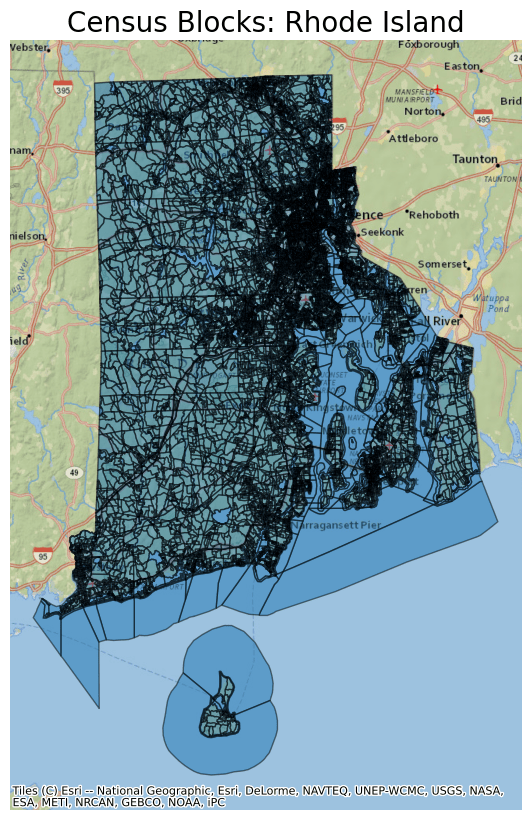
Both the geo and population tables use GEOID as a unique identifier, so the geometries and population data can be joined together. Remember that population data are not available for territories, so we'll use an inner join.
ri = (
    geo.get_partition(39)
    .compute()
    .join(pop[["P0010001"]].get_partition(39).compute(), how="inner")
)
ri = ri[ri.P0010001 > 10]
Now lets plot the census blocks in Providence County with at least 150 people.
providence = ri[(ri.P0010001 >= 150) & (ri.COUNTYFP == "007")]

ax = providence.to_crs(epsg=3857).plot(figsize=(10, 10), alpha=0.5, edgecolor="k")
ax.set_title(
    "Census Blocks with Population Greater than 150: Providence County, RI",
    fontdict={"fontsize": "20", "fontweight": "2"},
)
ctx.add_basemap(ax, source=ctx.providers.Esri.NatGeoWorldMap)
ax.set_axis_off()
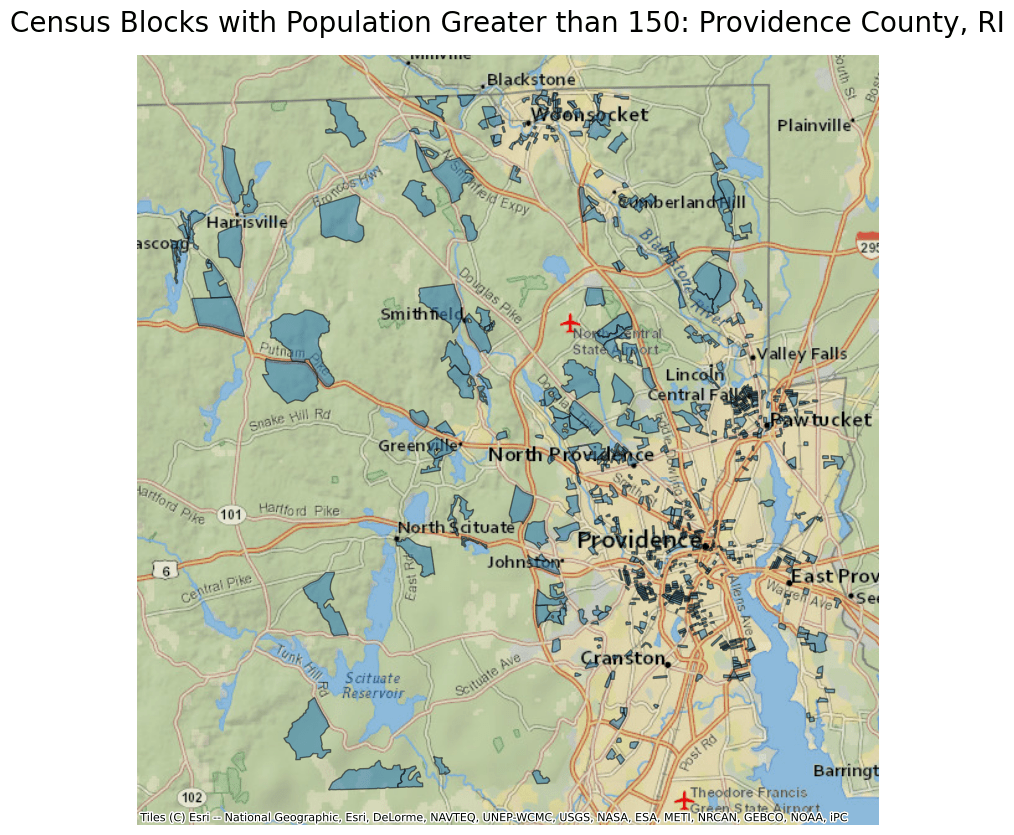
You can use this method with any census block within any county in the US.
Census data by cartographic boundaries
The second block of data is organized by different cartographic categories. These boundaries cover larger areas than the individual census blocks discussed above. The different categories range from census block groups (consisting of several census blocks) all the way up to a National Boundary file (encompassing the entire USA).
The files in this second group tend to be smaller in size than the census block data in the first group. Therefore, the files in the second group are not partitioned into multiple files, and each dataset only consists of one parquet file. Another difference is that the datasets in this second group include different information than the census block files in the first group and do not contain population statistics. Which additional data is included differs from dataset to dataset. See Appendix E. in the 2020 TIGER/Line Technical Documentation for more details on the available feature classes.
The following sections are examples of how to access and view each cartographic boundary file in this second group of data. Each example uses the same basic workflow and dependencies as the Census Block Boundaries for the first group of data. An important thing to note when using this data is that before plotting the data onto a basemap, the datasets need to be converted to Web Mercator (EPSG 3857) using the to_crs function of GeoPandas.
Some of the datasets are grouped together based on their type. It is important to note that some of the files may have gaps where no relevant data exists because states with no Tribal Block Groups do not have any Tribal Block Group data. The header for each example also includes the relevant abbreviation used for data access and retrieval.
American Indian Area Geographies
American Indian Area Geographies is the first grouping of cartographic boundary files available.
American Indian/Alaska Native Areas/Hawaiian Home Lands (AIANNH)
This file contains data for legal and statistical American Indian/Alaska Native Areas/Hawaiian Home Lands (AIANNH) entities published by the US Census Bureau.
The attribute table contains the following information:
- AIANNHCE = AIANNH census code
- AFFGEOID = American FactFinder summary level code + geovariant code + "00US" + GEOID
- GEOID = concatenation of AIANNH census code and reservation/statistical area or off-reservation trust land Hawaiian home land indicator
- NAME = Current Area Name
- NAMELSAD = Current name and legal/statistical status for each entity
- LSAD = Current legal/statistical area code
- ALAND = Current land area
- AWATER = Current water area
- geometry = coordinates for AIANNH polygons
Use the read_parquet function of Dask-GeoPandas to read the AIANNH data from the parquet file of the Planetary Computer dataset:
asset = census.get_item("2020-cb_2020_us_aiannh_500k").assets["data"]
ddf = geopandas.read_parquet(
    asset.href, storage_options=asset.extra_fields["table:storage_options"]
)
ddf.head()
| AIANNHCE | AIANNHNS | AFFGEOID | GEOID | NAME | NAMELSAD | LSAD | ALAND | AWATER | geometry | |
|---|---|---|---|---|---|---|---|---|---|---|
| 0 | 9515 | 2418775 | 2500000US9515 | 9515 | Apache Choctaw | Apache Choctaw SDTSA | 92 | 221751364 | 2632531 | POLYGON ((-93.77547 31.61937, -93.77411 31.619... |
| 1 | 9370 | 979494 | 2500000US9370 | 9370 | Shinnecock | Shinnecock (state) Reservation | 86 | 3494292 | 0 | POLYGON ((-72.44070 40.87749, -72.43870 40.879... |
| 2 | 9820 | 2418693 | 2500000US9820 | 9820 | MaChis Lower Creek | MaChis Lower Creek SDTSA | 92 | 1680767035 | 6816074 | MULTIPOLYGON (((-85.54654 31.21440, -85.54342 ... |
| 3 | 6125 | 2418774 | 2500000US6125 | 6125 | Anvik | Anvik ANVSA | 79 | 24578643 | 6308736 | POLYGON ((-160.24545 62.69478, -160.24517 62.6... |
| 4 | 6350 | 2418836 | 2500000US6350 | 6350 | Circle | Circle ANVSA | 79 | 274634016 | 1398608 | POLYGON ((-144.38284 65.73496, -144.37907 65.7... |
Next, plot the data from this parquet file and apply a basemap. Rather than displaying the whole dataset, show only the Apache Choctaw American Indian Homeland by selecting a subset of the dataframe where the values in the NAME column match "Apache Choctaw".
ddf = ddf.to_crs(epsg=3857)

ax = ddf[ddf.NAME == "Apache Choctaw"].plot(figsize=(10, 10), alpha=0.5, edgecolor="k")
ax.set_title(
    "Apache Choctaw American Indian Home Land",
    fontdict={"fontsize": "20", "fontweight": "2"},
)
ctx.add_basemap(ax, source=ctx.providers.Esri.NatGeoWorldMap)
ax.set_axis_off()
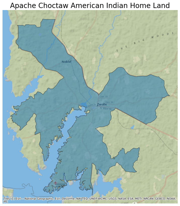
This map shows the shape of the Apache Choctaw American Indian Homeland overlaid on a Stamen Terrain Style basemap. To display the entire dataset, remove the part of the code that limits the dataframe to only the Apache Choctaw homeland. To plot a different area, change the dataframe's filter to a different attribute or value.
American Indian Tribal Subdivisions (AITSN)
This file contains data on American Indian Tribal Subdivisions. These areas are the legally defined subdivisions of American Indian Reservations (AIR), Oklahoma Tribal Statistical Areas (OTSA), and Off-Reservation Trust Land (ORTL).
The attribute table contains the following information:
- AIANNHCE = AIANNH census code
- TRSUBCE = Current AITSN census code
- TRSUBNS = ANSI feature code for American Indian Tribal Subdivision
- AFFGEOID = American FactFinder summary level code + geovariant code + "00US" + GEOID
- GEOID = concatenation of AIANNH census code and AITSN census code
- NAME = Current Area Name
- NAMELSAD = Current name and legal/statistical AITSN description
- LSAD = Current legal/statistical area code
- ALAND = Current land area
- AWATER = Current water area
- geometry = coordinates for AITSN polygons
Use the read_parquet function of Dask-GeoPandas to read the AIANNH data from the parquet file of the Planetary Computer dataset:
asset = census.get_item("2020-cb_2020_us_aitsn_500k").assets["data"]

ddf = geopandas.read_parquet(
    asset.href, storage_options=asset.extra_fields["table:storage_options"]
)
ddf.head()
| AIANNHCE | TRSUBCE | TRSUBNS | AFFGEOID | GEOID | NAME | NAMELSAD | LSAD | ALAND | AWATER | geometry | |
|---|---|---|---|---|---|---|---|---|---|---|---|
| 0 | 335 | 100 | 2418904 | 2510000US0335100 | 0335100 | Deer Creek | Deer Creek Segment | T3 | 91039385 | 1744201 | POLYGON ((-93.59601 47.89783, -93.57287 47.898... |
| 1 | 1150 | 400 | 2418959 | 2510000US1150400 | 1150400 | Hays | Hays District | 07 | 795597488 | 2961386 | MULTIPOLYGON (((-108.90981 47.91399, -108.8883... |
| 2 | 1160 | 300 | 2419007 | 2510000US1160300 | 1160300 | Mandaree | Mandaree Segment | T3 | 919294747 | 148670196 | POLYGON ((-102.78425 47.67410, -102.78497 47.7... |
| 3 | 5590 | 750 | 2418886 | 2510000US5590750 | 5590750 | 10 | County District 10 | TC | 3302876506 | 41402950 | POLYGON ((-96.45392 34.19828, -96.45372 34.257... |
| 4 | 5590 | 150 | 2418889 | 2510000US5590150 | 5590150 | 2 | County District 2 | TC | 2166517795 | 72598055 | POLYGON ((-95.04677 34.41936, -95.00595 34.419... |
Next, plot the data from this parquet file and overlay it on a basemap.
ddf.crs = 4326
ddf = ddf.to_crs(epsg=3857)

ax = ddf.plot(figsize=(10, 10), alpha=0.5, edgecolor="k")
ax.set_title(
    "American Indian Tribal Subdivisions",
    fontdict={"fontsize": "20", "fontweight": "2"},
)
ctx.add_basemap(ax, source=ctx.providers.Esri.NatGeoWorldMap)
ax.set_axis_off()
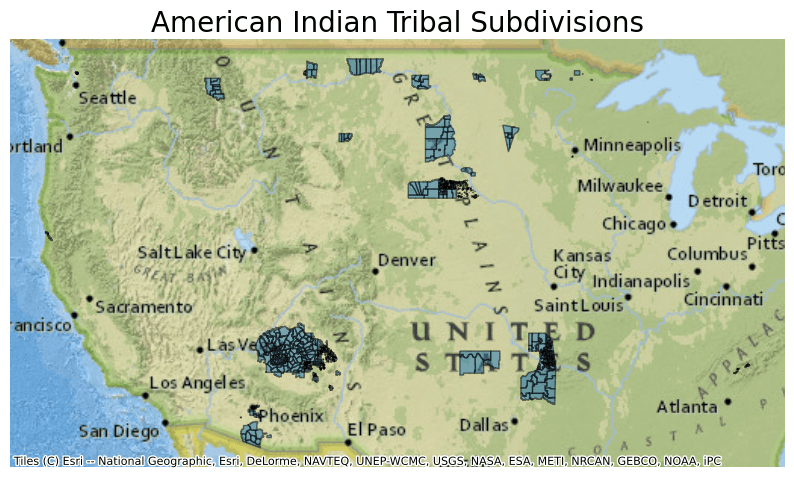
The map created shows all the American Indian Tribal Subdivisions.
Alaska Native Regional Corporations (ANRC)
This file contains data on Alaska Native Regional Corporations, which are corporations created according to the Alaska Native Claims Settlement Act.
The attribute table contains the following information:
- STATEFP = State FIPS code
- ANRCFP = ANRC FIPS code
- ANRCNS = ANSI feature code for Alaska Native Regional Corporation
- AFFGEOID American FactFinder summary level code + geovariant code + "00US" + GEOID
- GEOID = concatenation of state FIPS code and ANRC FIPS Code
- NAME = Current area name
- NAMELSAD = Current name and legal/statistical area description
- LSAD = Legal/statistical area description code
- ALAND = Current land area
- AWATER = Current water area
- geometry = coordinates for ANRC polygon
Use the read_parquet function of Dask-GeoPandas to read the ANRC data from the parquet file of the Planetary Computer dataset:
asset = census.get_item("2020-cb_2020_02_anrc_500k").assets["data"]
ddf = geopandas.read_parquet(
    asset.href, storage_options=asset.extra_fields["table:storage_options"]
)
ddf.head()
| STATEFP | ANRCFP | ANRCNS | AFFGEOID | GEOID | NAME | NAMELSAD | LSAD | ALAND | AWATER | geometry | |
|---|---|---|---|---|---|---|---|---|---|---|---|
| 0 | 02 | 9040 | 2419321 | 2300000US0209040 | 0209040 | Bristol Bay | Bristol Bay Alaska Native Regional Corporation | 77 | 104110270640 | 25993444733 | MULTIPOLYGON (((-158.15947 56.14452, -158.1537... |
| 1 | 02 | 590 | 2419295 | 2300000US0200590 | 0200590 | Ahtna | Ahtna Alaska Native Regional Corporation | 77 | 74027413736 | 1391256190 | POLYGON ((-149.38382 63.35746, -148.96463 63.4... |
| 2 | 02 | 67940 | 2419136 | 2300000US0267940 | 0267940 | Sealaska | Sealaska Alaska Native Regional Corporation | 77 | 91073660613 | 41754708205 | MULTIPOLYGON (((-132.09854 56.07761, -132.0974... |
| 3 | 02 | 17140 | 2418878 | 2300000US0217140 | 0217140 | Cook Inlet | Cook Inlet Alaska Native Regional Corporation | 77 | 96361403418 | 20418982039 | MULTIPOLYGON (((-150.28586 61.12704, -150.2808... |
| 4 | 02 | 9800 | 2419328 | 2300000US0209800 | 0209800 | Calista | Calista Alaska Native Regional Corporation | 77 | 142464876475 | 19389800572 | MULTIPOLYGON (((-161.67073 58.56075, -161.6672... |
Next, plot the data from this parquet file and overlay it on a basemap. To make the data work better with the Mercator Projection, exclude part of the dataset from the plot. To do so, limit your dataframe to rows that do not include "Aleut" in the AIANNHCE column.
ddf.crs = 4326
ddf = ddf.to_crs(epsg=3857)

ax = ddf[ddf.NAME != "Aleut"].plot(figsize=(10, 10), alpha=0.5, edgecolor="k")
ax.set_title(
    "Alaska Native Regional Corporations (excluding Aleut)",
    fontdict={"fontsize": "20", "fontweight": "2"},
)
ctx.add_basemap(ax, source=ctx.providers.Esri.NatGeoWorldMap)
ax.set_axis_off()
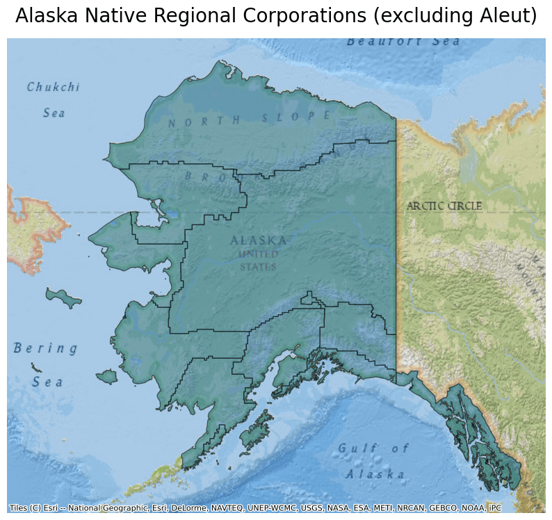
The map created shows all the Alaskan Native Regional Corporations except for Aleut.
Tribal Block Groups (TBG)
This file includes data on Tribal Block Groups, which are subdivisions of Tribal Census Tracts. These block groups can extend over multiple AIRs and ORTLs due to areas not meeting Block Group minimum population thresholds.
The attribute table contains the following information:
- AIANNHCE = AIANNH census code
- TTRACTCE = Tribal Census Tract Code
- TBLKGPCE = Tribal Block Group letter
- AFFGEOID = American FactFinder summary level code + geovariant code + "00US" + GEOID
- GEOID = concatenation of AIANNH census code, trivial census tract code, and tribal block group letter
- NAMELSAD = Current legal/statistical description and tribal block group letter
- LSAD = Current legal/statistical area code
- ALAND = Current land area
- AWATER = Current water area
- geometry = coordinates for Block Group polygons
Use the read_parquet function of Dask-GeoPandas to read the Tribal Block Group data from the parquet file of the Planetary Computer dataset:
asset = census.get_item("2020-cb_2020_us_tbg_500k").assets["data"]
ddf = geopandas.read_parquet(
    asset.href, storage_options=asset.extra_fields["table:storage_options"]
)
ddf.head()
| AIANNHCE | TTRACTCE | TBLKGPCE | AFFGEOID | GEOID | NAMELSAD | LSAD | ALAND | AWATER | geometry | |
|---|---|---|---|---|---|---|---|---|---|---|
| 0 | 2430 | T03700 | C | 2580000US2430T03700C | 2430T03700C | Tribal Block Group C | IB | 3945195 | 0 | POLYGON ((-111.26008 36.10715, -111.25910 36.1... |
| 1 | 20 | T00400 | B | 2580000US0020T00400B | 0020T00400B | Tribal Block Group B | IB | 1200584 | 100165 | POLYGON ((-116.47052 33.78691, -116.46940 33.7... |
| 2 | 1150 | T00100 | C | 2580000US1150T00100C | 1150T00100C | Tribal Block Group C | IB | 654354613 | 2911122 | MULTIPOLYGON (((-108.90981 47.91399, -108.8883... |
| 3 | 2555 | T01000 | A | 2580000US2555T01000A | 2555T01000A | Tribal Block Group A | IB | 39634390 | 4216784 | POLYGON ((-75.91155 43.00678, -75.90228 43.006... |
| 4 | 275 | T00100 | A | 2580000US0275T00100A | 0275T00100A | Tribal Block Group A | IB | 482651 | 0 | POLYGON ((-122.88954 39.02367, -122.88639 39.0... |
Next, plot the data from this parquet file and overlay it on a basemap. For this example, select only data for Tribal Block Group A by filtering by the TBLKGPCE column. Due to block group population threshold minimums, Tribal Block Group A spans a large portion of the contiguous United States and is not fully connected.
ddf.crs = 4326
ddf = ddf.to_crs(epsg=3857)

ax = ddf[ddf.TBLKGPCE == "A"].plot(figsize=(10, 10), alpha=0.5, edgecolor="k")
ax.set_title(
    "Tribal Block Group A",
    fontdict={"fontsize": "20", "fontweight": "2"},
)
ctx.add_basemap(ax, source=ctx.providers.Esri.NatGeoWorldMap)
ax.set_axis_off()
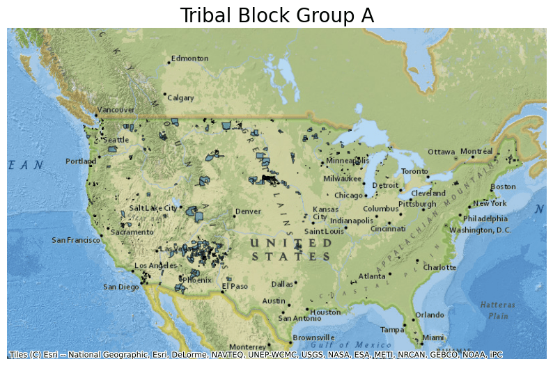
The map created shows Tribal Block Group A.
Tribal Census Tracts (TTRACT)
This file includes data on Tribal Census Tracts which are relatively small statistical subdivisions of AIRs and ORTLs defined by federally recognized tribal government officials in partnership with the Census Bureau. Due to population thresholds, the Tracts may consist of multiple non-contiguous areas.
The attribute table contains the following information:
- AIANNHCE = AIANNH census code
- TTRACTCE = Tribal Census Tract Code
- AFFGEOID = American FactFinder summary level code + geovariant code + "00US" + GEOID
- GEOID = concatenation of AIANNH census code and tribal census tract code
- NAME = Tribal Census Tract name
- NAMELSAD = Current legal/statistical description and tribal census tract name
- LSAD = Current legal/statistical area code
- ALAND = Current land area
- AWATER = Current water area
- geometry = coordinates for Tribal Census Tract polygons
Use the read_parquet function of Dask-GeoPandas to read the Tribal Block Group data from the parquet file of the Planetary Computer dataset:
asset = census.get_item("2020-cb_2020_us_ttract_500k").assets["data"]
ddf = geopandas.read_parquet(
    asset.href, storage_options=asset.extra_fields["table:storage_options"]
)
ddf.head()
| AIANNHCE | TTRACTCE | AFFGEOID | GEOID | NAME | NAMELSAD | LSAD | ALAND | AWATER | geometry | |
|---|---|---|---|---|---|---|---|---|---|---|
| 0 | 990 | T00100 | 2560000US0990T00100 | 0990T00100 | T001 | Tribal Census Tract T001 | IT | 134672514 | 47477 | MULTIPOLYGON (((-83.38715 35.46808, -83.38610 ... |
| 1 | 3935 | T00100 | 2560000US3935T00100 | 3935T00100 | T001 | Tribal Census Tract T001 | IT | 614259770 | 20267661 | MULTIPOLYGON (((-98.76648 48.00405, -98.76471 ... |
| 2 | 1160 | T00200 | 2560000US1160T00200 | 1160T00200 | T002 | Tribal Census Tract T002 | IT | 1955706500 | 421434881 | POLYGON ((-102.65466 47.87091, -102.65497 47.8... |
| 3 | 525 | T00100 | 2560000US0525T00100 | 0525T00100 | T001 | Tribal Census Tract T001 | IT | 4176988 | 0 | MULTIPOLYGON (((-80.89902 34.90259, -80.89470 ... |
| 4 | 4390 | T00100 | 2560000US4390T00100 | 4390T00100 | T001 | Tribal Census Tract T001 | IT | 1612375179 | 5684784 | POLYGON ((-110.53722 40.44993, -110.53444 40.4... |
Next, plot the data from this parquet file and overlay it on a basemap. For this example, select only data for Tribal Census Tract T002 by filtering by the NAME column. Due to census tract population threshold minimums, Tribal Census Tract T002 spans a large portion of the contiguous United States and is not fully connected.
ddf.crs = 4326
ddf = ddf.to_crs(epsg=3857)

ax = ddf[ddf.NAME == "T002"].plot(figsize=(10, 10), alpha=0.5, edgecolor="k")
ax.set_title(
    "Tribal Census Tract T002",
    fontdict={"fontsize": "20", "fontweight": "2"},
)
ctx.add_basemap(ax, source=ctx.providers.Esri.NatGeoWorldMap)
ax.set_axis_off()
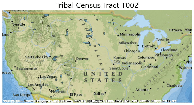
The map created shows Tribal Census Tract T002.
Census Block Groups (BG)
This file contains data on Census Block Groups. These groups are the second smallest geographic grouping. They consist of clusters of blocks within the same census tract that share the same first digit of their 4-character census block number. Census Block Groups generally contain between 600 and 3,000 people and generally cover contiguous areas.
The attribute table contains the following information:
- STATEFP = State FIPS code
- COUNTYFP = County FIPS code
- TRACTCE = Census tract code
- BLKGRPCE = Block group number
- AFFGEOID = American FactFinder summary level code + geovariant code + "00US" + GEOID
- GEOID = Concatenation of State FIPS, County FIPS, Census tract code, and block group number
- NAME = Block group number
- NAMELSAD = Legal/statistical description and group number
- LSAD = Legal/statistical classification
- ALAND = Current land area
- AWATER = Current water area
- geometry = coordinates for Block Group polygons
Use the read_parquet function of Dask-GeoPandas to read the Block Group data from the parquet file of the Planetary Computer dataset:
asset = census.get_item("2020-cb_2020_us_bg_500k").assets["data"]
ddf = geopandas.read_parquet(
    asset.href, storage_options=asset.extra_fields["table:storage_options"]
)
ddf.head()
| STATEFP | COUNTYFP | TRACTCE | BLKGRPCE | AFFGEOID | GEOID | NAME | NAMELSAD | LSAD | ALAND | AWATER | geometry | |
|---|---|---|---|---|---|---|---|---|---|---|---|---|
| 0 | 36 | 029 | 4200 | 2 | 1500000US360290042002 | 360290042002 | 2 | Block Group 2 | BG | 168802 | 0 | POLYGON ((-78.81870 42.93591, -78.81814 42.936... |
| 1 | 36 | 061 | 12400 | 8 | 1500000US360610124008 | 360610124008 | 8 | Block Group 8 | BG | 18510 | 0 | POLYGON ((-73.95425 40.76617, -73.95203 40.765... |
| 2 | 36 | 059 | 410400 | 4 | 1500000US360594104004 | 360594104004 | 4 | Block Group 4 | BG | 305990 | 0 | POLYGON ((-73.72361 40.66781, -73.72217 40.672... |
| 3 | 36 | 047 | 118800 | 2 | 1500000US360471188002 | 360471188002 | 2 | Block Group 2 | BG | 52033 | 0 | POLYGON ((-73.86754 40.68043, -73.86575 40.680... |
| 4 | 36 | 005 | 12500 | 1 | 1500000US360050125001 | 360050125001 | 1 | Block Group 1 | BG | 100794 | 0 | POLYGON ((-73.89529 40.82814, -73.89506 40.828... |
Next, plot the data from this parquet file and overlay it on a basemap. For this example, select only data for the state of California by filtering by the State FIPS code ("06") in the STATEFP column.
ddf.crs = 4326
ddf = ddf.to_crs(epsg=3857)

ax = ddf[ddf.STATEFP == "06"].plot(figsize=(10, 10), alpha=0.5, edgecolor="k")
ax.set_title(
    "Census Block Groups: California",
    fontdict={"fontsize": "20", "fontweight": "2"},
)
ctx.add_basemap(ax, source=ctx.providers.Esri.NatGeoWorldMap)
ax.set_axis_off()
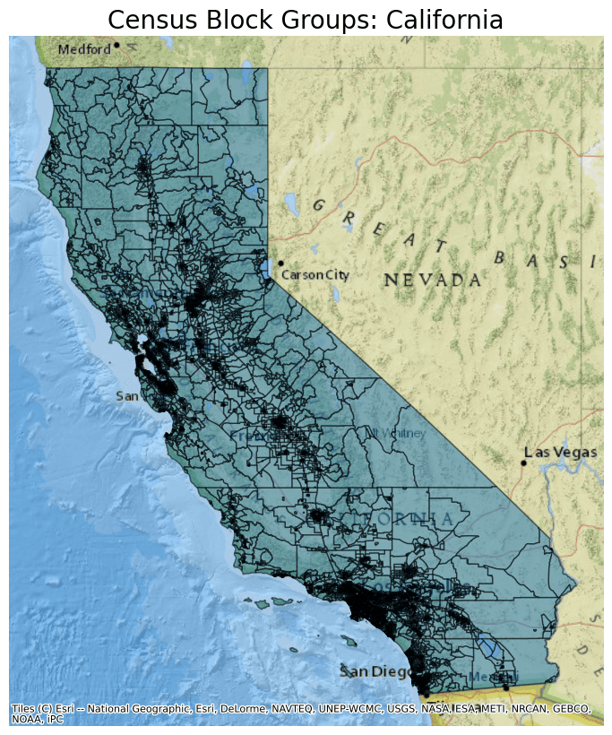
The map created shows all the Census Block Groups in California.
Census Tracts (TRACT)
This file contains data on Census Tracts which are small and relatively permanent statistical subdivisions of a county or equivalent entity. Tract population size is generally between 1,200 and 8,000 people with an ideal size of 4,000. Boundaries tend to follow visible and identifiable features and are usually contiguous areas.
The attribute table contains the following information:
- STATEFP = State FIPS code
- COUNTYFP = County FIPS code
- TRACTCE = Census tract code
- AFFGEOID = American FactFinder summary level code + geovariant code + "00US" + GEOID
- GEOID = Concatenation of State FIPS, County FIPS, and Census tract code
- NAME = Census Tract name, it is the census tract code converted to an integer
- NAMELSAD = Legal/statistical description and tract name
- STUSPS = FIPS State Postal Code
- NAMELSADCO = County name
- STATE_NAME = State Name
- LSAD = Legal/statistical classification
- ALAND = Current land area
- AWATER = Current water area
- geometry = coordinates for Census Tract polygons
Use the read_parquet function of Dask-GeoPandas to read the Census Tract data from the parquet file of the Planetary Computer dataset:
asset = census.get_item("2020-cb_2020_us_tract_500k").assets["data"]
ddf = geopandas.read_parquet(
    asset.href, storage_options=asset.extra_fields["table:storage_options"]
)
ddf.head()
| STATEFP | COUNTYFP | TRACTCE | AFFGEOID | GEOID | NAME | NAMELSAD | STUSPS | NAMELSADCO | STATE_NAME | LSAD | ALAND | AWATER | geometry | |
|---|---|---|---|---|---|---|---|---|---|---|---|---|---|---|
| 0 | 17 | 089 | 853004 | 1400000US17089853004 | 17089853004 | 8530.04 | Census Tract 8530.04 | IL | Kane County | Illinois | CT | 3622334 | 91650 | POLYGON ((-88.35003 41.80764, -88.34938 41.810... |
| 1 | 11 | 001 | 5003 | 1400000US11001005003 | 11001005003 | 50.03 | Census Tract 50.03 | DC | District of Columbia | District of Columbia | CT | 94136 | 0 | POLYGON ((-77.03195 38.90965, -77.03032 38.909... |
| 2 | 06 | 037 | 482503 | 1400000US06037482503 | 06037482503 | 4825.03 | Census Tract 4825.03 | CA | Los Angeles County | California | CT | 729678 | 0 | POLYGON ((-118.09949 34.06262, -118.09466 34.0... |
| 3 | 31 | 153 | 10630 | 1400000US31153010630 | 31153010630 | 106.30 | Census Tract 106.30 | NE | Sarpy County | Nebraska | CT | 4964876 | 0 | POLYGON ((-96.23429 41.19035, -96.23010 41.190... |
| 4 | 12 | 057 | 13706 | 1400000US12057013706 | 12057013706 | 137.06 | Census Tract 137.06 | FL | Hillsborough County | Florida | CT | 535141 | 10298 | POLYGON ((-82.34769 27.89656, -82.34680 27.898... |
Next, plot the data from this parquet file and overlay it on a basemap. For this example, select only data for Census Tracts located in Washington, DC by filtering for "DC" in the STUSPS column.
ddf.crs = 4326
ddf = ddf.to_crs(epsg=3857)

ax = ddf[ddf.STUSPS == "DC"].plot(figsize=(10, 10), alpha=0.5, edgecolor="k")
ax.set_title(
    "Census Tracts: Washington, DC",
    fontdict={"fontsize": "20", "fontweight": "2"},
)
ctx.add_basemap(ax, source=ctx.providers.Esri.NatGeoWorldMap)
ax.set_axis_off()
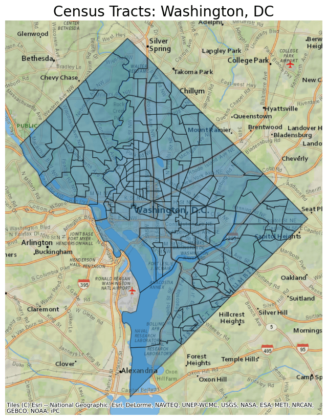
The map created shows all the Census Tracts in Washington, DC.
Congressional Districts: 116th Congress (CD116)
This file contains data on the Congressional Districts for the 116th Congress.
The attribute table contains the following information:
- STATEFP = State FIPS Code
- CD116FP = Congressional District FIPS code
- AFFGEOID = American FactFinder summary level code + geovariant code + "00US" + GEOID
- GEOID = Concatenation of State FIPS and congressional district FIPS code
- NAMELSAD = Legal/statistical description and name
- LSAD = Legal/statistical classification
- CDSESSN = Congressional Session Code
- ALAND = Current land area
- AWATER = Current water area
- geometry = coordinates for Congressional District polygons
Use the read_parquet function of Dask-GeoPandas to read the Congressional District data from the parquet file of the Planetary Computer dataset:
asset = census.get_item("2020-cb_2020_us_cd116_500k").assets["data"]
ddf = geopandas.read_parquet(
    asset.href, storage_options=asset.extra_fields["table:storage_options"]
)
ddf.head()
| STATEFP | CD116FP | AFFGEOID | GEOID | NAMELSAD | LSAD | CDSESSN | ALAND | AWATER | geometry | |
|---|---|---|---|---|---|---|---|---|---|---|
| 0 | 06 | 42 | 5001600US0642 | 0642 | Congressional District 42 | C2 | 116 | 2424753563 | 44105315 | POLYGON ((-117.67629 33.88882, -117.65488 33.8... |
| 1 | 39 | 7 | 5001600US3907 | 3907 | Congressional District 7 | C2 | 116 | 10010016396 | 64562455 | MULTIPOLYGON (((-82.55933 40.78975, -82.55835 ... |
| 2 | 48 | 3 | 5001600US4803 | 4803 | Congressional District 3 | C2 | 116 | 1245574011 | 97890112 | POLYGON ((-96.84410 32.98891, -96.84403 32.992... |
| 3 | 28 | 2 | 5001600US2802 | 2802 | Congressional District 2 | C2 | 116 | 40278711117 | 951654563 | POLYGON ((-91.36371 31.78036, -91.35951 31.799... |
| 4 | 42 | 18 | 5001600US4218 | 4218 | Congressional District 18 | C2 | 116 | 757655195 | 19985421 | POLYGON ((-80.17834 40.33725, -80.17537 40.338... |
Next, plot the data from this parquet file and overlay it on a basemap. For this example, select only data for Maryland"s 2nd Congressional District by filtering by the State FIPS code 24 and the Congressional District FIPS code 02 in the GEOID column.
ddf.crs = 4326
ddf = ddf.to_crs(epsg=3857)

ax = ddf[ddf.GEOID == "2402"].plot(figsize=(10, 10), alpha=0.5, edgecolor="k")
ax.set_title(
    "2nd Congressional District: Maryland",
    fontdict={"fontsize": "20", "fontweight": "2"},
)
ctx.add_basemap(ax, source=ctx.providers.Esri.NatGeoWorldMap)
ax.set_axis_off()
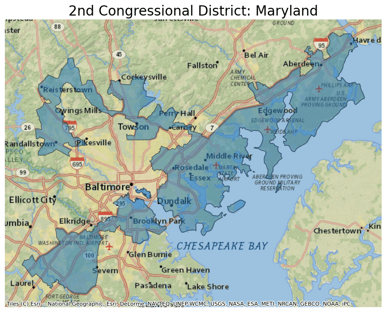
The map created shows Maryland"s 2nd Congressional District.
Consolidated Cities (CONCITY)
This file contains data on Consolidated Cities. These are areas where one or several other incorporated places in a county or Minor Civil Division are included in a consolidated government but still exist as separate legal entities.
The attribute table contains the following information:
- STATEFP = State FIPS Code
- CONCTYFP = Consolidated city FIPS code
- CONCTYNS = Consolidated city GNIS code
- AFFGEOID = American FactFinder summary level code + geovariant code + "00US" + GEOID
- GEOID = Concatenation of State FIPS and consolidated city FIPS code
- NAME = Consolidated city name
- NAMELSAD = Name and Legal/statistical description
- LSAD = Legal/statistical classification
- ALAND = Current land area
- AWATER = Current water area
- geometry = coordinates for Consolidated City polygons
Use the read_parquet function of Dask-GeoPandas to read the Consolidated City data from the parquet file of the Planetary Computer dataset:
asset = census.get_item("2020-cb_2020_us_concity_500k").assets["data"]
ddf = geopandas.read_parquet(
    asset.href, storage_options=asset.extra_fields["table:storage_options"]
)
ddf.head()
| STATEFP | CONCTYFP | CONCTYNS | AFFGEOID | GEOID | NAME | NAMELSAD | LSAD | ALAND | AWATER | geometry | |
|---|---|---|---|---|---|---|---|---|---|---|---|
| 0 | 20 | 28410 | 2664357 | 1700000US2028410 | 2028410 | Greeley County | Greeley County unified government | UG | 2015424640 | 0 | POLYGON ((-102.04526 38.50540, -102.04526 38.5... |
| 1 | 13 | 3436 | 2407404 | 1700000US1303436 | 1303436 | Athens-Clarke County | Athens-Clarke County unified government | UG | 308784927 | 4688313 | POLYGON ((-83.53739 33.96591, -83.49824 33.987... |
| 2 | 30 | 11390 | 2409651 | 1700000US3011390 | 3011390 | Butte-Silver Bow | Butte-Silver Bow | 00 | 1859568271 | 1518178 | POLYGON ((-113.08552 45.86065, -113.08282 45.8... |
| 3 | 21 | 48003 | 1967435 | 1700000US2148003 | 2148003 | Louisville/Jefferson County | Louisville/Jefferson County metro government | MT | 986271740 | 43513298 | POLYGON ((-85.94711 38.00509, -85.94222 38.007... |
| 4 | 09 | 47500 | 2378334 | 1700000US0947500 | 0947500 | Milford | Milford city | 25 | 57444044 | 10216676 | POLYGON ((-73.12245 41.18290, -73.12137 41.187... |
Next, plot the data from this parquet file and overlay it on a basemap. For this example, select only data for Athens-Clarke County, GA, which is a Consolidated City. Select the data by filtering by the NAME column.
ddf.crs = 4326
ddf = ddf.to_crs(epsg=3857)

ax = ddf[ddf.NAME == "Athens-Clarke County"].plot(
    figsize=(10, 10), alpha=0.5, edgecolor="k"
)
ax.set_title(
    "Consolidated City: Athens-Clarke County, GA",
    fontdict={"fontsize": "20", "fontweight": "2"},
)
ctx.add_basemap(ax, source=ctx.providers.Esri.NatGeoWorldMap)
ax.set_axis_off()
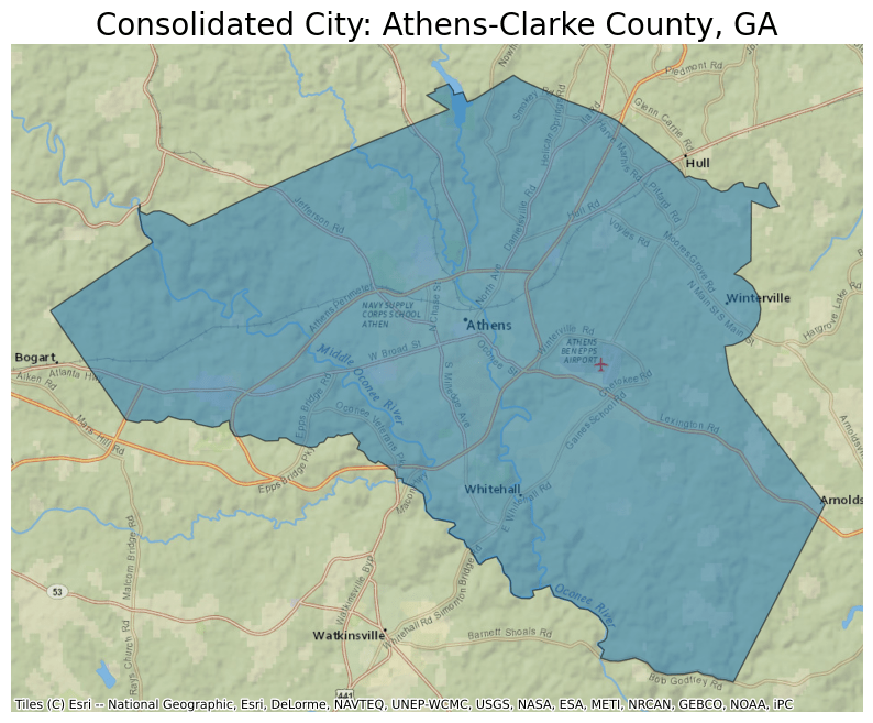
The map created shows Athens-Clarke County, GA.
Counties (COUNTY)
This file contains data on Counties and Equivalent Entities. These are the primary legal divisions of states. Most states use the term "counties," but other terms such as "Parishes," "Municipios," or "Independent Cities" may be used.
The attribute table contains the following information:
- STATEFP = State FIPS Code
- COUNTYFP = County FIPS code
- COUNTNS = ANSI feature code for the county
- AFFGEOID = American FactFinder summary level code + geovariant code + "00US" + GEOID
- GEOID = Concatenation of State FIPS and county FIPS code
- NAME = County name
- NAMELSAD = Name and Legal/statistical description
- STUSPS = FIPS State Postal Code
- LSAD = Legal/statistical classification
- ALAND = Current land area
- AWATER = Current water area
- geometry = coordinates for County polygons
Use the read_parquet function of Dask-GeoPandas to read the Counties and Equivalent Entities data from the parquet file of the Planetary Computer dataset:
asset = census.get_item("2020-cb_2020_us_county_500k").assets["data"]
ddf = geopandas.read_parquet(
    asset.href, storage_options=asset.extra_fields["table:storage_options"]
)
ddf.head()
| STATEFP | COUNTYFP | COUNTYNS | AFFGEOID | GEOID | NAME | NAMELSAD | STUSPS | STATE_NAME | LSAD | ALAND | AWATER | geometry | |
|---|---|---|---|---|---|---|---|---|---|---|---|---|---|
| 0 | 21 | 141 | 00516917 | 0500000US21141 | 21141 | Logan | Logan County | KY | Kentucky | 06 | 1430224002 | 12479211 | POLYGON ((-87.06037 36.68085, -87.06002 36.708... |
| 1 | 36 | 081 | 00974139 | 0500000US36081 | 36081 | Queens | Queens County | NY | New York | 06 | 281594050 | 188444349 | POLYGON ((-73.96262 40.73903, -73.96243 40.739... |
| 2 | 34 | 017 | 00882278 | 0500000US34017 | 34017 | Hudson | Hudson County | NJ | New Jersey | 06 | 119640822 | 41836491 | MULTIPOLYGON (((-74.04220 40.69997, -74.03900 ... |
| 3 | 34 | 019 | 00882228 | 0500000US34019 | 34019 | Hunterdon | Hunterdon County | NJ | New Jersey | 06 | 1108086284 | 24761598 | POLYGON ((-75.19511 40.57969, -75.19466 40.581... |
| 4 | 21 | 147 | 00516926 | 0500000US21147 | 21147 | McCreary | McCreary County | KY | Kentucky | 06 | 1105416696 | 10730402 | POLYGON ((-84.77845 36.60329, -84.73068 36.665... |
Next, plot the data from this parquet file and overlay it on a basemap. For this example, select only data for counties in Minnesota by filtering by the STATE_NAME column.
ddf.crs = 4326
ddf = ddf.to_crs(epsg=3857)

ax = ddf[ddf.STATE_NAME == "Minnesota"].plot(figsize=(10, 10), alpha=0.5, edgecolor="k")
ax.set_title(
    "Minnesota: Counties",
    fontdict={"fontsize": "20", "fontweight": "2"},
)
ctx.add_basemap(ax, source=ctx.providers.Esri.NatGeoWorldMap)
ax.set_axis_off()
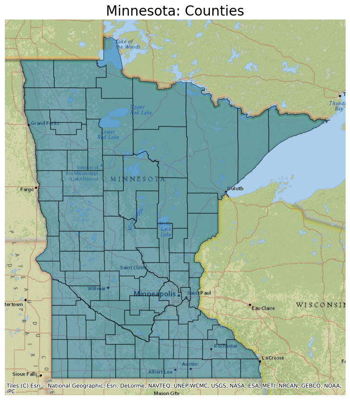
The map created shows Minnesota Counties.
Counties within Congressional Districts: 116th Congress (COUNTY_within_CD116)
This file contains data on Counties within Congressional Districts.
The attribute PARTFLG identifies whether all or only part of a County is within a Congressional District:
- N = All of a County is within a Congressional District
- Y = only part of a county is within a Congressional District
The attribute table contains the following information:
- STATEFP = State FIPS code
- COUNTYFP = County FIPS code
- CD116FP = Congressional District FIPS code
- AFFGEOID = American FactFinder summary level code + geovariant code + "00US" + GEOID
- GEOID = Concatenation of State FIPS, Congressional District FIPS, and county FIPS code
- PARTFLD = Identifies if all or part of entity is within the file
- ALAND = Current Land Area
- geometry = coordinates for polygons
Use the read_parquet function of Dask-GeoPandas to read the Counties within Congressional Districts data from the parquet file of the Planetary Computer dataset:
asset = census.get_item("2020-cb_2020_us_county_within_cd116_500k").assets["data"]
ddf = geopandas.read_parquet(
    asset.href, storage_options=asset.extra_fields["table:storage_options"]
)
ddf.head()
| STATEFP | COUNTYFP | CD116FP | AFFGEOID | GEOID | PARTFLG | ALAND | geometry | |
|---|---|---|---|---|---|---|---|---|
| 0 | 05 | 057 | 4 | 5101600US0504057 | 0504057 | N | 1883438547 | POLYGON ((-93.96945 33.74021, -93.96842 33.741... |
| 1 | 54 | 037 | 2 | 5101600US5402037 | 5402037 | N | 542072983 | POLYGON ((-78.03545 39.27822, -78.03326 39.279... |
| 2 | 02 | 170 | 0 | 5101600US0200170 | 0200170 | N | 63990747114 | POLYGON ((-153.00188 62.72583, -152.99961 62.7... |
| 3 | 54 | 013 | 2 | 5101600US5402013 | 5402013 | N | 723253605 | POLYGON ((-81.27841 38.91487, -81.27417 38.918... |
| 4 | 12 | 077 | 2 | 5101600US1202077 | 1202077 | N | 2164099094 | POLYGON ((-85.15381 30.09285, -85.15185 30.094... |
Next, plot the data from this parquet file and overlay it on a basemap. For this example, select only polygons where only part of the County is within a Congressional District. Select the relevant data by filtering by "Y" in the PARTFLG column.
ddf.crs = 4326
ddf = ddf.to_crs(epsg=3857)

ax = ddf[ddf.PARTFLG == "Y"].plot(figsize=(20, 10), alpha=0.5, edgecolor="k")
ax.set_title(
    "Counties only partially within a Congressional Districts",
    fontdict={"fontsize": "30", "fontweight": "2"},
)
ctx.add_basemap(ax, source=ctx.providers.Esri.NatGeoWorldMap)
ax.set_axis_off()
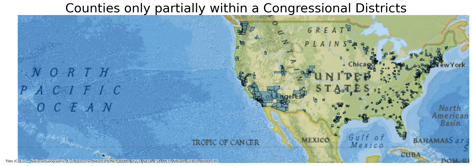
The map created shows Counties partially within Congressional Districts.
County Subdivisions (COUSUB)
This file contains County Subdivisions, which are the primary divisions of counties and equivalent entities. These divisions vary from state to state and include Barrios, Purchases, Townships, and other types of legal and statistical entities.
The attribute table contains the following information:
- STATEFP = State FIPS code
- COUNTYFP = County FIPS code
- COUSUBFP = Subdivision FIPS code
- COUSUBNS = ANSI feature for the subdivision
- AFFGEOID = American FactFinder summary level code + geovariant code + "00US" + GEOID
- GEOID = Concatenation of State FIPS, county FIPS, and county subdivision FIPS
- NAME = Subdivision name
- NAMELSAD = Subdivision name and legal/statistical description
- STUSPS = FIPS State Postal Code
- NAMELSADCO = County name
- STATE_NAME = State Name
- LSAD = Legal/statistical classification
- ALAND = Current land area
- AWATER = Current water area
- geometry = coordinates for County Subdivision polygons
Use the read_parquet function of Dask-GeoPandas to read the County Subdivisions data from the parquet file of the Planetary Computer dataset:
asset = census.get_item("2020-cb_2020_us_cousub_500k").assets["data"]
ddf = geopandas.read_parquet(
    asset.href, storage_options=asset.extra_fields["table:storage_options"]
)
ddf.head()
| STATEFP | COUNTYFP | COUSUBFP | COUSUBNS | AFFGEOID | GEOID | NAME | NAMELSAD | STUSPS | NAMELSADCO | STATE_NAME | LSAD | ALAND | AWATER | geometry | |
|---|---|---|---|---|---|---|---|---|---|---|---|---|---|---|---|
| 0 | 42 | 117 | 52960 | 01217118 | 0600000US4211752960 | 4211752960 | Nelson | Nelson township | PA | Tioga County | Pennsylvania | 44 | 29020811 | 25916 | POLYGON ((-77.31788 41.97075, -77.31029 41.970... |
| 1 | 46 | 109 | 42820 | 01268550 | 0600000US4610942820 | 4610942820 | Minnesota | Minnesota township | SD | Roberts County | South Dakota | 44 | 121465694 | 3383863 | POLYGON ((-97.10387 45.90342, -97.10309 45.908... |
| 2 | 46 | 083 | 20780 | 01267387 | 0600000US4608320780 | 4608320780 | Fairview | Fairview town | SD | Lincoln County | South Dakota | 43 | 221380 | 0 | POLYGON ((-96.49153 43.22389, -96.48526 43.224... |
| 3 | 47 | 009 | 91340 | 02464659 | 0600000US4700991340 | 4700991340 | 8 | District 8 | TN | Blount County | Tennessee | 28 | 646087619 | 509512 | POLYGON ((-83.99881 35.55556, -83.99444 35.558... |
| 4 | 48 | 489 | 93435 | 01939169 | 0600000US4848993435 | 4848993435 | San Perlita | San Perlita CCD | TX | Willacy County | Texas | 22 | 739156645 | 483409952 | MULTIPOLYGON (((-97.25810 26.42544, -97.25596 ... |
Next, plot the data from this parquet file and overlay it on a basemap. For this example, plot all the subdivisions, townships in this case, in Bergen County, NJ. Select the relevant data by filtering by the NAMELSADCO column.
ddf.crs = 4326
ddf = ddf.to_crs(epsg=3857)

ax = ddf[ddf.NAMELSADCO == "Bergen County"].plot(
    figsize=(10, 10), alpha=0.5, edgecolor="k"
)
ax.set_title(
    "County Subdivisions: Bergen County, NJ",
    fontdict={"fontsize": "20", "fontweight": "2"},
)
ctx.add_basemap(ax, source=ctx.providers.Esri.NatGeoWorldMap)
ax.set_axis_off()
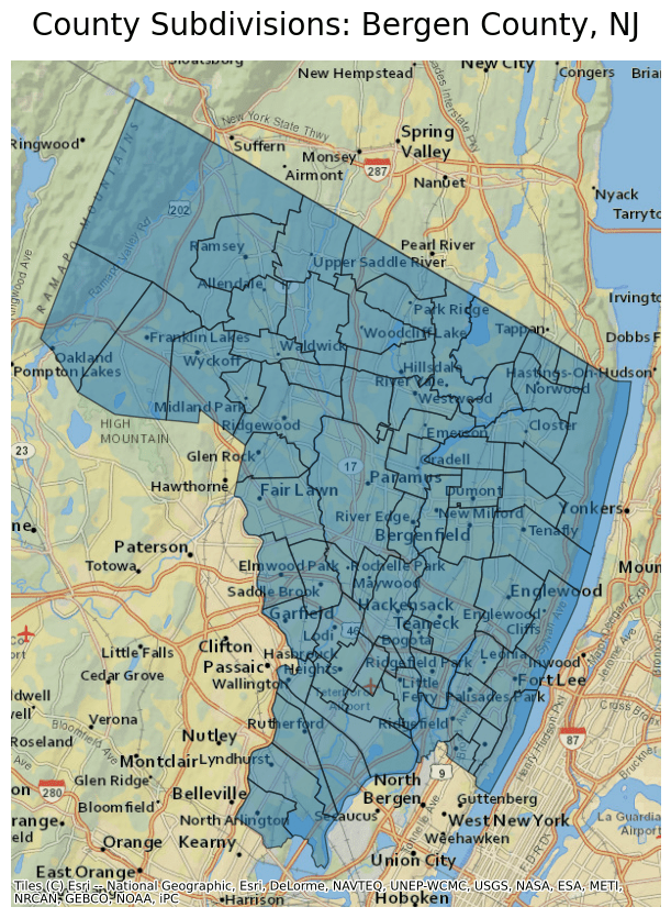
The map created shows County Subdivisions in Bergen County, NJ.
Divisions (DIVISION)
This file contains data on Divisions of the US. This file is similar to the Regions file but contains more divisions and encompasses several states per division.
The attribute table contains the following information:
- DIVISIONCE = Number assigned to each division
- AFFGEOID = American FactFinder summary level code + geovariant code + "00US" + GEOID
- GEOID = DIVISIONCE
- NAME = Name of division
- NAMELSAD = Division name and legal/statistical description
- LSAD = Legal/statistical classification
- ALAND = Current land area
- AWATER = Current water area
- geometry = coordinates for Division polygons
Use the read_parquet function of Dask-GeoPandas to read the Division data from the parquet file of the Planetary Computer dataset:
asset = census.get_item("2020-cb_2020_us_division_500k").assets["data"]
ddf = geopandas.read_parquet(
    asset.href, storage_options=asset.extra_fields["table:storage_options"]
)
ddf.head()
| DIVISIONCE | AFFGEOID | GEOID | NAME | NAMELSAD | LSAD | ALAND | AWATER | geometry | |
|---|---|---|---|---|---|---|---|---|---|
| 0 | 5 | 0300000US5 | 5 | South Atlantic | South Atlantic Division | 69 | 687125298338 | 86339601557 | MULTIPOLYGON (((-75.56555 39.51485, -75.56174 ... |
| 1 | 3 | 0300000US3 | 3 | East North Central | East North Central Division | 69 | 629298010339 | 151248789139 | MULTIPOLYGON (((-82.73447 41.60351, -82.72425 ... |
| 2 | 4 | 0300000US4 | 4 | West North Central | West North Central Division | 69 | 1314700010733 | 33034200327 | MULTIPOLYGON (((-89.59206 47.96668, -89.59147 ... |
| 3 | 8 | 0300000US8 | 8 | Mountain | Mountain Division | 69 | 2217352931824 | 19266522413 | POLYGON ((-120.00574 39.22866, -120.00567 39.2... |
| 4 | 9 | 0300000US9 | 9 | Pacific | Pacific Division | 69 | 2319992840165 | 296172644163 | MULTIPOLYGON (((-139.51201 59.70289, -139.5095... |
Next, plot the data from this parquet file and overlay it on a basemap. For this example, select only data from the Mountain division by filtering by the NAME column.
ddf.crs = 4326
ddf = ddf.to_crs(epsg=3857)

ax = ddf[ddf.NAME == "Mountain"].plot(figsize=(10, 10), alpha=0.5, edgecolor="k")
ax.set_title(
    "Divisions: Mountain Region",
    fontdict={"fontsize": "20", "fontweight": "2"},
)
ctx.add_basemap(ax, source=ctx.providers.Esri.NatGeoWorldMap)
ax.set_axis_off()
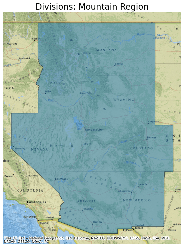
The map created shows the Mountain Region Division.
Metropolitan and Micropolitan Statistical Areas and Related Statistical Areas
Metropolitan and Micropolitan Statistical Areas and Related Statistical Areas is the second grouping of datasets within the census data by cartographic boundaries group. A metropolitan or micropolitan statistical area contains a core area, with a substantial population with adjacent communities having a high degree of economic and social integration with that core. This grouping contains six datasets.
Core Based Statistical Areas (CBSAs)
This file contains data on Core Based Statistical Areas (CBSAs). This encompasses all metropolitan and micropolitan statistical areas.
The attribute table contains the following information:
- CSAFP = Combined statistical area code (if applicable)
- CBSAFP = Metropolitan statistical area/micropolitan statistical area code
- AFFGEOID = American FactFinder summary level code + geovariant code + "00US" + GEOID
- GEOID = CBSAFP
- NAME = Metropolitan statistical area/micropolitan statistical area name
- NAMELSAD = CBSA name and legal/statistical description
- LSAD = Legal/statistical classification
- ALAND = Current land area
- AWATER = Current water area
- geometry = coordinates for CBSA polygons
Use the read_parquet function of Dask-GeoPandas to read the CBSA data from the parquet file of the Planetary Computer dataset:
asset = census.get_item("2020-cb_2020_us_cbsa_500k").assets["data"]
ddf = geopandas.read_parquet(
    asset.href, storage_options=asset.extra_fields["table:storage_options"]
)
ddf.head()
| CSAFP | CBSAFP | AFFGEOID | GEOID | NAME | NAMELSAD | LSAD | ALAND | AWATER | geometry | |
|---|---|---|---|---|---|---|---|---|---|---|
| 0 | <NA> | 11380 | 310M600US11380 | 11380 | Andrews, TX | Andrews, TX Micro Area | M2 | 3886850259 | 957039 | POLYGON ((-103.06470 32.52219, -103.00047 32.5... |
| 1 | 192 | 35140 | 310M600US35140 | 35140 | Newberry, SC | Newberry, SC Micro Area | M2 | 1632452022 | 44011454 | POLYGON ((-81.94372 34.20605, -81.94196 34.208... |
| 2 | <NA> | 37540 | 310M600US37540 | 37540 | Paris, TN | Paris, TN Micro Area | M2 | 1455320362 | 81582236 | POLYGON ((-88.52940 36.17018, -88.52636 36.229... |
| 3 | 246 | 29900 | 310M600US29900 | 29900 | Laurinburg, NC | Laurinburg, NC Micro Area | M2 | 826569986 | 3842049 | POLYGON ((-79.69251 34.80685, -79.68822 34.809... |
| 4 | 315 | 35460 | 310M600US35460 | 35460 | Newport, TN | Newport, TN Micro Area | M2 | 1129584563 | 17932684 | POLYGON ((-83.31519 35.89332, -83.31078 35.895... |
Next, plot the data from this parquet file and overlay it on a basemap. For this example, select Kahului-Wailuku-Lahaina, HI Metro Area by filtering by the NAME column.
ddf.crs = 4326
ddf = ddf.to_crs(epsg=3857)

ax = ddf[ddf.NAME == "Kahului-Wailuku-Lahaina, HI"].plot(
    figsize=(10, 10), alpha=0.5, edgecolor="k"
)
ax.set_title(
    "Core Based Statistical Area: Kahului-Wailuku-Lahaina, HI Metro Area",
    fontdict={"fontsize": "20", "fontweight": "2"},
)
ctx.add_basemap(ax, source=ctx.providers.Esri.NatGeoWorldMap)
ax.set_axis_off()
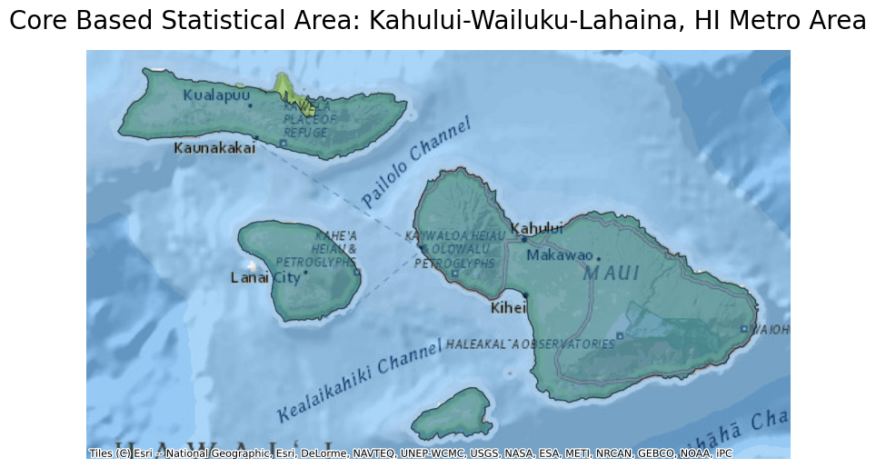
The map created shows the Kahului-Wailuku-Lahaina, HI Metro Area, Core Based Statistical Area.
Combined Statistical Areas (CSA)
This file contains data on Combined Statistical Areas, which are areas that consist of two or more adjacent CBSAs that have significant employment interchanges.
The attribute table contains the following information:
- CSAFP = Combined statistical area code
- AFFGEOID = American FactFinder summary level code + geovariant code + "00US" + GEOID
- GEOID = CSAFP
- NAME = CSA Name
- NAMELSAD = CSA name and legal/statistical description
- LSAD = Legal/statistical classification
- ALAND = Current land area
- AWATER = Current water area
- geometry = coordinates for CSA polygons
Use the read_parquet function of Dask-GeoPandas to read the CSA data from the parquet file of the Planetary Computer dataset:
asset = census.get_item("2020-cb_2020_us_csa_500k").assets["data"]
ddf = geopandas.read_parquet(
    asset.href, storage_options=asset.extra_fields["table:storage_options"]
)
ddf.head()
| CSAFP | AFFGEOID | GEOID | NAME | NAMELSAD | LSAD | ALAND | AWATER | geometry | |
|---|---|---|---|---|---|---|---|---|---|
| 0 | 146 | 330M600US146 | 146 | Bloomsburg-Berwick-Sunbury, PA | Bloomsburg-Berwick-Sunbury, PA CSA | M0 | 4444039108 | 86464626 | POLYGON ((-77.36418 40.84694, -77.27924 40.909... |
| 1 | 368 | 330M600US368 | 368 | Memphis-Forrest City, TN-MS-AR | Memphis-Forrest City, TN-MS-AR CSA | M0 | 13493874541 | 322004792 | POLYGON ((-91.15230 34.92548, -91.15074 34.968... |
| 2 | 356 | 330M600US356 | 356 | Macon-Bibb County--Warner Robins, GA | Macon-Bibb County--Warner Robins, GA CSA | M0 | 5827265752 | 49165153 | POLYGON ((-84.20263 32.69002, -84.19676 32.701... |
| 3 | 290 | 330M600US290 | 290 | Huntsville-Decatur, AL | Huntsville-Decatur, AL CSA | M0 | 6816635309 | 269975554 | POLYGON ((-87.53028 34.45756, -87.53011 34.469... |
| 4 | 206 | 330M600US206 | 206 | Dallas-Fort Worth, TX-OK | Dallas-Fort Worth, TX-OK CSA | M0 | 40234482778 | 1682397922 | POLYGON ((-98.57613 32.57248, -98.57600 32.624... |
Next, plot the data from this parquet file and overlay it on a basemap. For this example, select the San Jose-San Francisco-Oakland CSA by filtering by the NAME column.
ddf.crs = 4326
ddf = ddf.to_crs(epsg=3857)

ax = ddf[ddf.NAME == "San Jose-San Francisco-Oakland, CA"].plot(
    figsize=(10, 10), alpha=0.5, edgecolor="k"
)
ax.set_title(
    "Combined Statistical Area: San Jose-San Francisco-Oakland, CA",
    fontdict={"fontsize": "20", "fontweight": "2"},
)
ctx.add_basemap(ax, source=ctx.providers.Esri.NatGeoWorldMap)
ax.set_axis_off()
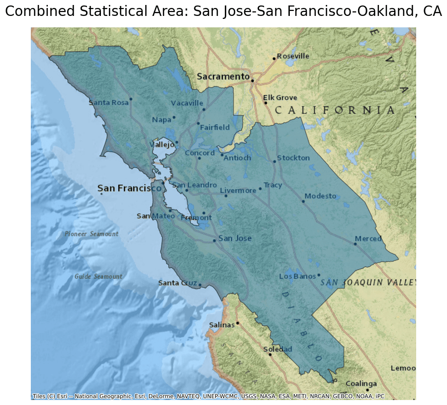
The map created shows the San Jose-San Francisco-Oakland, CA Combined Statistical Area.
Metropolitan Divisions (METDIV)
This file contains data on Metropolitan Divisions. These areas are groupings of counties or equivalent entities within a metropolitan statistical area with a core of 2.5 million inhabitants and one or more main counties that represent employment centers, plus adjacent counties with commuting ties.
The attribute table contains the following information:
- CSAFP = Combined statistical area code
- CBSAFP = Metropolitan statistical area/micropolitan statistical area code
- METDIVFP = Metropolitan division code
- AFFGEOID = American FactFinder summary level code + geovariant code + "00US" + GEOID
- GEOID = Concatenation of CBSAFP and METDIVFP
- NAME = Metropolitan division name
- NAMELSAD = MetDiv name and legal/statistical description
- LSAD = Legal/statistical classification
- ALAND = Current land area
- AWATER = Current water area
- geometry = coordinates for Metropolitan Division polygons
Use the read_parquet function of Dask-GeoPandas to read the Metropolitan Division data from the parquet file of the Planetary Computer dataset:
asset = census.get_item("2020-cb_2020_us_metdiv_500k").assets["data"]
ddf = geopandas.read_parquet(
    asset.href, storage_options=asset.extra_fields["table:storage_options"]
)
ddf.head()
| CSAFP | CBSAFP | METDIVFP | AFFGEOID | GEOID | NAME | NAMELSAD | LSAD | ALAND | AWATER | geometry | |
|---|---|---|---|---|---|---|---|---|---|---|---|
| 0 | 348 | 31080 | 11244 | 314M600US3108011244 | 3108011244 | Anaheim-Santa Ana-Irvine, CA | Anaheim-Santa Ana-Irvine, CA Metro Division | M3 | 2053449483 | 406294114 | POLYGON ((-118.11442 33.74518, -118.11305 33.7... |
| 1 | 148 | 14460 | 14454 | 314M600US1446014454 | 1446014454 | Boston, MA | Boston, MA Metro Division | M3 | 2882301581 | 1411559356 | MULTIPOLYGON (((-70.88335 42.34049, -70.88158 ... |
| 2 | 148 | 14460 | 15764 | 314M600US1446015764 | 1446015764 | Cambridge-Newton-Framingham, MA | Cambridge-Newton-Framingham, MA Metro Division | M3 | 3393859579 | 945476893 | MULTIPOLYGON (((-70.58029 42.63602, -70.57509 ... |
| 3 | 428 | 37980 | 15804 | 314M600US3798015804 | 3798015804 | Camden, NJ | Camden, NJ Metro Division | M3 | 3477449505 | 108072755 | POLYGON ((-75.42830 39.78437, -75.42168 39.787... |
| 4 | 176 | 16980 | 16984 | 314M600US1698016984 | 1698016984 | Chicago-Naperville-Evanston, IL | Chicago-Naperville-Evanston, IL Metro Division | M3 | 8106981077 | 1895152877 | POLYGON ((-88.70738 42.49359, -88.67080 42.494... |
Next, plot the data from this parquet file and overlay it on a basemap. For this example, select out Chicago-Naperville-Evanston, IL Metropolitan Divisions by filtering by the NAME column.
ddf.crs = 4326
ddf = ddf.to_crs(epsg=3857)

ax = ddf[ddf.NAME == "Chicago-Naperville-Evanston, IL"].plot(
    figsize=(10, 10), alpha=0.5, edgecolor="k"
)
ax.set_title(
    "Metropolitan Divisions: Chicago-Naperville-Evanston, IL",
    fontdict={"fontsize": "20", "fontweight": "2"},
)
ctx.add_basemap(ax, source=ctx.providers.Esri.NatGeoWorldMap)
ax.set_axis_off()
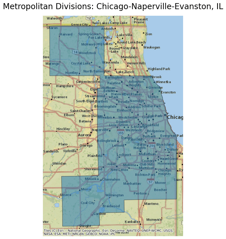
The map created shows Metropolitan Divisions in Illinois and Indiana.
New England City and Town Areas (NECTA)
This file contains New England City and Town Areas, which encompass metropolitan and micropolitan statistical areas and urban clusters in New England.
The attribute table contains the following information:
- CNECTAFP = Combined NECTA code
- NECTAFP = NECTA code
- AFFGEOID = American FactFinder summary level code + geovariant code + "00US" + GEOID
- GEOID = NECTAFP
- NAME = NECTA name
- NAMELSAD = NECTA name and legal/statistical description
- LSAD = Legal/statistical classification
- ALAND = Current land area
- AWATER = Current water area
- geometry = coordinates for New England City and Town Area polygons
Use the read_parquet function of Dask-GeoPandas to read the New England City and Town Areas data from the parquet file of the Planetary Computer dataset:
asset = census.get_item("2020-cb_2020_us_necta_500k").assets["data"]
ddf = geopandas.read_parquet(
    asset.href, storage_options=asset.extra_fields["table:storage_options"]
)
ddf.head()
| CNECTAFP | NECTAFP | AFFGEOID | GEOID | NAME | NAMELSAD | LSAD | ALAND | AWATER | geometry | |
|---|---|---|---|---|---|---|---|---|---|---|
| 0 | 790 | 73300 | 350M600US73300 | 73300 | Greenfield Town, MA | Greenfield Town, MA Micropolitan NECTA | M6 | 576790797 | 12695651 | POLYGON ((-72.85766 42.73761, -72.80911 42.736... |
| 1 | 725 | 72500 | 350M600US72500 | 72500 | Claremont, NH | Claremont, NH Micropolitan NECTA | M6 | 207547766 | 2886013 | POLYGON ((-72.41538 43.38021, -72.41315 43.384... |
| 2 | NaN | 73050 | 350M600US73050 | 73050 | Dover-Durham, NH-ME | Dover-Durham, NH-ME Metropolitan NECTA | M5 | 1153772202 | 38371631 | POLYGON ((-71.24697 43.27619, -71.23601 43.284... |
| 3 | NaN | 78500 | 350M600US78500 | 78500 | Vineyard Haven, MA | Vineyard Haven, MA Micropolitan NECTA | M6 | 233141285 | 675399599 | MULTIPOLYGON (((-70.83204 41.25950, -70.82983 ... |
| 4 | 715 | 74500 | 350M600US74500 | 74500 | Leominster-Gardner, MA | Leominster-Gardner, MA Metropolitan NECTA | M5 | 1028154238 | 65184023 | POLYGON ((-72.31363 42.39640, -72.31509 42.398... |
Next, plot all polygons from this parquet file and overlay all of the New England City and Town Areas on a basemap.
ddf.crs = 4326
ddf = ddf.to_crs(epsg=3857)

ax = ddf.plot(figsize=(10, 10), alpha=0.5, edgecolor="k")
ax.set_title(
    "New England City and Town Areas",
    fontdict={"fontsize": "20", "fontweight": "2"},
)
ctx.add_basemap(ax, source=ctx.providers.Esri.NatGeoWorldMap)
ax.set_axis_off()
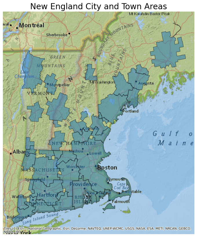
The map created shows New England City and Town Areas.
New England City and Town Area Division (NECTADIV)
This file contains New England City and Town Areas Divisions, which are smaller groupings of cities and towns in New England that contain a single core of 2.5 million inhabitants. Each division must have a total population of 100,000 or more.
The attribute table contains the following information:
- CNECTAFP = Combined NECTA code
- NECTAFP = NECTA code
- NCTADVFP = NECTA Division code
- AFFGEOID = American FactFinder summary level code + geovariant code + "00US" + GEOID
- GEOID = Concatenation of NECTA code and NECT division code
- NAME = NECTA Division name
- NAMELSAD = NECTA Division name and legal/statistical description
- LSAD = Legal/statistical classification
- ALAND = Current land area
- AWATER = Current water area
- geometry = coordinates for New England City and Town Area Division polygons
Use the read_parquet function of Dask-GeoPandas to read the New England City and Town Areas Divisions data from the parquet file of the Planetary Computer dataset:
asset = census.get_item("2020-cb_2020_us_nectadiv_500k").assets["data"]
ddf = geopandas.read_parquet(
    asset.href, storage_options=asset.extra_fields["table:storage_options"]
)
ddf.head()
| CNECTAFP | NECTAFP | NCTADVFP | AFFGEOID | GEOID | NAME | NAMELSAD | LSAD | ALAND | AWATER | geometry | |
|---|---|---|---|---|---|---|---|---|---|---|---|
| 0 | 715 | 71650 | 78254 | 355M600US7165078254 | 7165078254 | Taunton-Middleborough-Norton, MA | Taunton-Middleborough-Norton, MA NECTA Division | M7 | 777613767 | 49344655 | POLYGON ((-71.25929 41.97422, -71.23516 41.983... |
| 1 | 715 | 71650 | 73604 | 355M600US7165073604 | 7165073604 | Haverhill-Newburyport-Amesbury Town, MA-NH | Haverhill-Newburyport-Amesbury Town, MA-NH NEC... | M7 | 938908432 | 56403579 | POLYGON ((-71.31096 42.93573, -71.30006 42.969... |
| 2 | 715 | 71650 | 74204 | 355M600US7165074204 | 7165074204 | Lawrence-Methuen Town-North Andover, MA-NH | Lawrence-Methuen Town-North Andover, MA-NH NEC... | M7 | 207887604 | 9753119 | POLYGON ((-71.28426 42.76011, -71.26375 42.785... |
| 3 | 715 | 71650 | 71634 | 355M600US7165071634 | 7165071634 | Boston-Cambridge-Newton, MA | Boston-Cambridge-Newton, MA NECTA Division | M7 | 2860356873 | 425756189 | MULTIPOLYGON (((-70.95108 42.28973, -70.94864 ... |
| 4 | 715 | 71650 | 72104 | 355M600US7165072104 | 7165072104 | Brockton-Bridgewater Town-Easton, MA | Brockton-Bridgewater Town-Easton, MA NECTA Div... | M7 | 321543380 | 7532122 | POLYGON ((-71.16747 42.06163, -71.14226 42.071... |
Next, plot all polygons from this parquet file and overlay all of the New England City and Town Area Divisions on a basemap.
ddf.crs = 4326
ddf = ddf.to_crs(epsg=3857)

ax = ddf.plot(figsize=(10, 10), alpha=0.5, edgecolor="k")
ax.set_title(
    "New England City and Town Area Divisions",
    fontdict={"fontsize": "20", "fontweight": "2"},
)
ctx.add_basemap(ax, source=ctx.providers.Esri.NatGeoWorldMap)
ax.set_axis_off()
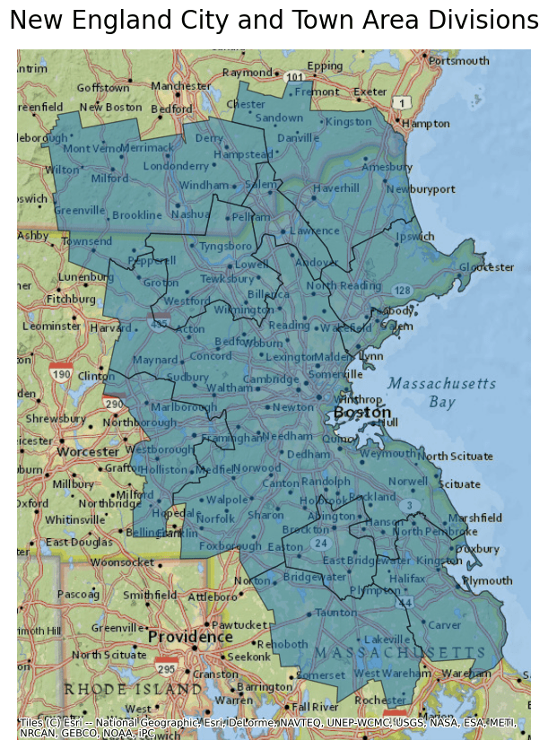
The map created shows New England City and Town Area Divisions.
Combined New England City and Town Areas (CNECTA)
This file contains data on Combined New England City and Town Areas, consisting of two or more adjacent NECTAs that have significant employment interchanges.
The attribute table contains the following information:
- CNECTAFP = Combined NECTA code
- AFFGEOID = American FactFinder summary level code + geovariant code + "00US" + GEOID
- GEOID = CNECTA
- NAME = Combined NECTA name
- NAMELSAD = Combined NECTA name and legal/statistical description
- LSAD = Legal/statistical classification
- ALAND = Current land area
- AWATER = Current water area
- geometry = coordinates for Combined New England City and Town Area polygons
Use the read_parquet function of Dask-GeoPandas to read the Combined New England City and Town Areas data from the parquet file of the Planetary Computer dataset:
asset = census.get_item("2020-cb_2020_us_cnecta_500k").assets["data"]
ddf = geopandas.read_parquet(
    asset.href, storage_options=asset.extra_fields["table:storage_options"]
)
ddf.head()
| CNECTAFP | AFFGEOID | GEOID | NAME | NAMELSAD | LSAD | ALAND | AWATER | geometry | |
|---|---|---|---|---|---|---|---|---|---|
| 0 | 710 | 335M600US710 | 710 | Augusta-Waterville, ME | Augusta-Waterville, ME Combined NECTA | M4 | 2155041281 | 183932221 | POLYGON ((-70.04529 44.49481, -70.04230 44.494... |
| 1 | 715 | 335M600US715 | 715 | Boston-Worcester-Providence, MA-RI-NH-CT-ME | Boston-Worcester-Providence, MA-RI-NH-CT-ME Co... | M4 | 21419143755 | 3004992276 | MULTIPOLYGON (((-70.58029 42.63602, -70.57509 ... |
| 2 | 720 | 335M600US720 | 720 | Bridgeport-New Haven-Stamford, CT | Bridgeport-New Haven-Stamford, CT Combined NECTA | M4 | 3939856869 | 374600689 | MULTIPOLYGON (((-72.76143 41.24233, -72.75973 ... |
| 3 | 725 | 335M600US725 | 725 | Lebanon-Claremont, NH-VT | Lebanon-Claremont, NH-VT Combined NECTA | M4 | 3032422367 | 58164272 | POLYGON ((-72.64469 43.79013, -72.62226 43.817... |
| 4 | 770 | 335M600US770 | 770 | Pittsfield-North Adams, MA-VT | Pittsfield-North Adams, MA-VT Combined NECTA | M4 | 1524388842 | 24505481 | POLYGON ((-73.40063 42.37903, -73.39156 42.403... |
Next, plot all polygons from this parquet file and overlay all of the Combined New England City and Town Areas on a basemap.
ddf.crs = 4326
ddf = ddf.to_crs(epsg=3857)

ax = ddf.plot(figsize=(10, 10), alpha=0.5, edgecolor="k")
ax.set_title(
    "Combined New England City and Town Areas",
    fontdict={"fontsize": "20", "fontweight": "2"},
)
ctx.add_basemap(ax, source=ctx.providers.Esri.NatGeoWorldMap)
ax.set_axis_off()
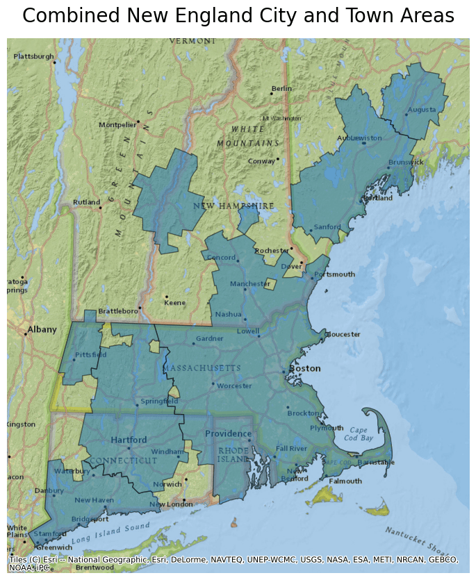
The map created shows Combined New England City and Town Areas.
Places (PLACE)
This file contains Places which are Incorporated Places (legal entities) and Census Designated Places (CDPs, statistical entities). An incorporated place usually is a city, town, village, or borough but can have other legal descriptions. CDPs are settled concentrations of population that are identifiable by name but are not legally incorporated.
The attribute table contains the following information:
- STATEFP = State FIPS code
- PLACEFP = Place FIPS code
- PLACENS = Place GNIS code
- AFFGEOID = American FactFinder summary level code + geovariant code + "00US" + GEOID
- GEOID = Concatenation of State FIPS code and Place FIPS code
- NAME = Place name
- NAMELSAD = Place name and legal/statistical description
- STUSPS = FIPS Postal code
- STATE_NAME = State name
- LSAD = Legal/statistical classification
- ALAND = Current land area
- AWATER = Current water area
- geometry = coordinates for Place polygons
Use the read_parquet function of Dask-GeoPandas to read the Places data from the parquet file of the Planetary Computer dataset:
asset = census.get_item("2020-cb_2020_us_place_500k").assets["data"]
ddf = geopandas.read_parquet(
    asset.href, storage_options=asset.extra_fields["table:storage_options"]
)
ddf.head()
| STATEFP | PLACEFP | PLACENS | AFFGEOID | GEOID | NAME | NAMELSAD | STUSPS | STATE_NAME | LSAD | ALAND | AWATER | geometry | |
|---|---|---|---|---|---|---|---|---|---|---|---|---|---|
| 0 | 12 | 28575 | 2403791 | 1600000US1228575 | 1228575 | Hampton | Hampton city | FL | Florida | 25 | 2728657 | 0 | POLYGON ((-82.15433 29.86419, -82.14682 29.864... |
| 1 | 12 | 625 | 2405131 | 1600000US1200625 | 1200625 | Alford | Alford town | FL | Florida | 43 | 2731534 | 49685 | POLYGON ((-85.40333 30.70450, -85.39543 30.704... |
| 2 | 12 | 26050 | 2406576 | 1600000US1226050 | 1226050 | Glen Ridge | Glen Ridge town | FL | Florida | 43 | 442668 | 54824 | POLYGON ((-80.08267 26.67634, -80.07902 26.676... |
| 3 | 13 | 69000 | 2405429 | 1600000US1369000 | 1369000 | Savannah | Savannah city | GA | Georgia | 25 | 276730651 | 12329738 | MULTIPOLYGON (((-81.23851 32.06725, -81.21279 ... |
| 4 | 13 | 67284 | 2404651 | 1600000US1367284 | 1367284 | Roswell | Roswell city | GA | Georgia | 25 | 105461127 | 3308483 | POLYGON ((-84.41903 34.06118, -84.41903 34.061... |
Next, plot the data from this parquet file and overlay it on a basemap. For this example, select all the Places in Washington State by filtering by "WA" in the STUSPS column.
ddf.crs = 4326
ddf = ddf.to_crs(epsg=3857)

ax = ddf[ddf.STUSPS == "WA"].plot(figsize=(10, 10), alpha=0.5, edgecolor="k")
ax.set_title(
    "Places: Washington State",
    fontdict={"fontsize": "20", "fontweight": "2"},
)
ctx.add_basemap(ax, source=ctx.providers.Esri.NatGeoWorldMap)
ax.set_axis_off()
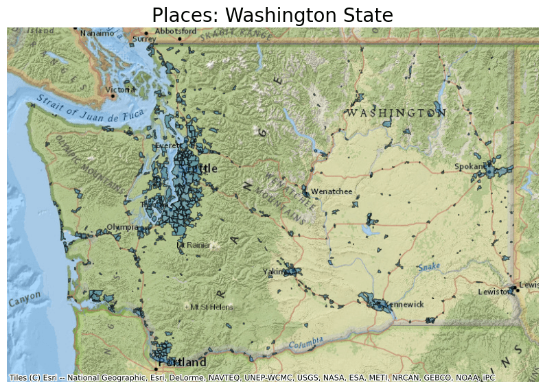
The map created shows Places in Washington State.
Regions (REGION)
This file contains Regions of the US and encompasses several states per division.
The attribute table contains the following information:
- REGIONCE = Number assigned to each Region
- AFFGEOID = American FactFinder summary level code + geovariant code + "00US" + GEOID
- GEOID = REGIONCE
- NAME = Name of region
- NAMELSAD = Region name and legal/statistical description
- LSAD = Legal/statistical classification
- ALAND = Current land area
- AWATER = Current water area
- geometry = coordinates for Region polygons
Use the read_parquet function of Dask-GeoPandas to read the Regions data from the parquet file of the Planetary Computer dataset:
asset = census.get_item("2020-cb_2020_us_region_500k").assets["data"]
ddf = geopandas.read_parquet(
    asset.href, storage_options=asset.extra_fields["table:storage_options"]
)
ddf.head()
| REGIONCE | AFFGEOID | GEOID | NAME | NAMELSAD | LSAD | ALAND | AWATER | geometry | |
|---|---|---|---|---|---|---|---|---|---|
| 0 | 3 | 0200000US3 | 3 | South | South Region | 68 | 2249827294436 | 148750821211 | MULTIPOLYGON (((-89.34216 30.05917, -89.33606 ... |
| 1 | 2 | 0200000US2 | 2 | Midwest | Midwest Region | 68 | 1943998021072 | 184282989466 | MULTIPOLYGON (((-82.73447 41.60351, -82.72425 ... |
| 2 | 4 | 0200000US4 | 4 | West | West Region | 68 | 4537345771989 | 315439166576 | MULTIPOLYGON (((-147.46941 60.92206, -147.4682... |
| 3 | 1 | 0200000US1 | 1 | Northeast | Northeast Region | 68 | 419355661549 | 50259697277 | MULTIPOLYGON (((-67.32260 44.61160, -67.32174 ... |
Next, plot the data from this parquet file and overlay it on a basemap. For this example, select the entire South Region by filtering by the NAME column.
ddf.crs = 4326
ddf = ddf.to_crs(epsg=3857)

ax = ddf[ddf.NAME == "South"].plot(figsize=(10, 10), alpha=0.5, edgecolor="k")
ax.set_title(
    "South Region",
    fontdict={"fontsize": "20", "fontweight": "2"},
)
ctx.add_basemap(ax, source=ctx.providers.Esri.NatGeoWorldMap)
ax.set_axis_off()
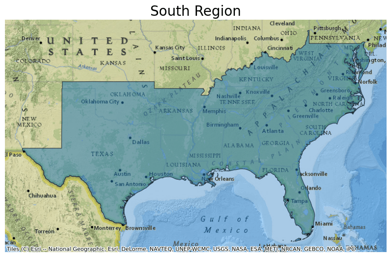
The map created shows the South Region.
School Districts
School Districts is the third grouping of datasets within the census data by cartographic boundaries group. This dataset grouping includes district boundaries for Elementary School Districts, Secondary School Districts, and Unified School Districts.
School Districts - Elementary (ELSD)
This file contains Elementary School Districts, referring to districts with elementary schools.
The attribute table contains the following information:
- STATEFP = State FIPS code
- ELSDLEA = Elementary School District local education agency code
- AFFGEOID = American FactFinder summary level code + geovariant code + "00US" + GEOID
- GEOID = Concatenation of State FIPS code and ELSDLEA code
- NAME = Elementary School District name
- STUSPS = FIPS Postal code
- STATE_NAME = State name
- LSAD = Legal/statistical classification
- ALAND = Current land area
- AWATER = Current water area
- geometry = coordinates for Elementary School District polygons
Use the read_parquet function of Dask-GeoPandas to read the Elementary School Districts data from the parquet file of the Planetary Computer dataset:
asset = census.get_item("2020-cb_2020_us_elsd_500k").assets["data"]
ddf = geopandas.read_parquet(
    asset.href, storage_options=asset.extra_fields["table:storage_options"]
)
ddf.head()
| STATEFP | ELSDLEA | AFFGEOID | GEOID | NAME | STUSPS | STATE_NAME | LSAD | ALAND | AWATER | geometry | |
|---|---|---|---|---|---|---|---|---|---|---|---|
| 0 | 17 | 42570 | 9500000US1742570 | 1742570 | Willow Springs School District 108 | IL | Illinois | 00 | 24565916 | 2685308 | POLYGON ((-87.91426 41.71660, -87.90923 41.719... |
| 1 | 40 | 4470 | 9500000US4004470 | 4004470 | Bishop Public School | OK | Oklahoma | 00 | 18936631 | 0 | POLYGON ((-98.44840 34.59449, -98.43973 34.594... |
| 2 | 17 | 8790 | 9500000US1708790 | 1708790 | Cass School District 63 | IL | Illinois | 00 | 11006857 | 329296 | POLYGON ((-88.00218 41.72823, -88.00230 41.729... |
| 3 | 34 | 5520 | 9500000US3405520 | 3405520 | Franklin Township School District | NJ | New Jersey | 00 | 60657041 | 232602 | POLYGON ((-75.10323 40.71943, -75.06000 40.753... |
| 4 | 17 | 17160 | 9500000US1717160 | 1717160 | Gower School District 62 | IL | Illinois | 00 | 13484773 | 437292 | POLYGON ((-87.96002 41.75215, -87.95929 41.752... |
Next, plot the data from this parquet file and overlay it on a basemap. For this example, select all the Elementary School Districts in Montana by filtering by "MT" in the STUSPS column.
ddf.crs = 4326
ddf = ddf.to_crs(epsg=3857)

ax = ddf[ddf.STUSPS == "MT"].plot(figsize=(10, 10), alpha=0.5, edgecolor="k")
ax.set_title(
    "Montana Elementary School Districts",
    fontdict={"fontsize": "20", "fontweight": "2"},
)
ctx.add_basemap(ax, source=ctx.providers.Esri.NatGeoWorldMap)
ax.set_axis_off()
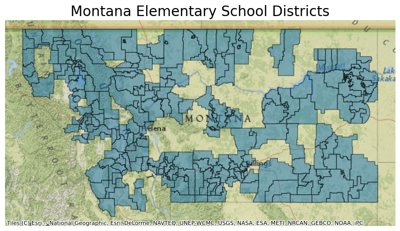
The map created shows the Montana Elementary School Districts.
School Districts - Secondary (SCSD)
This file contains Secondary School Districts, referring to districts with secondary schools.
The attribute table contains the following information:
- STATEFP = State FIPS code
- SCDLEA = Secondary School District local education agency code
- AFFGEOID = American FactFinder summary level code + geovariant code + "00US" + GEOID
- GEOID = Concatenation of State FIPS code and SCSDLEA code
- NAME = Secondary School District name
- STUSPS = FIPS Postal code. STATE_NAME = State name
- LSAD = Legal/statistical classification
- ALAND = Current land area
- AWATER = Current water area
- geometry = Coordinates for Secondary School District polygons
Use the read_parquet function of Dask-GeoPandas to read the Secondary School Districts data from the parquet file of the Planetary Computer dataset:
asset = census.get_item("2020-cb_2020_us_scsd_500k").assets["data"]
ddf = geopandas.read_parquet(
    asset.href, storage_options=asset.extra_fields["table:storage_options"]
)
ddf.head()
| STATEFP | SCSDLEA | AFFGEOID | GEOID | NAME | STUSPS | STATE_NAME | LSAD | ALAND | AWATER | geometry | |
|---|---|---|---|---|---|---|---|---|---|---|---|
| 0 | 06 | 99004 | 9600000US0699004 | 0699004 | Sierra Unified School District (9-12) | CA | California | 00 | 2950629174 | 63592439 | POLYGON ((-119.40472 37.09651, -119.39820 37.0... |
| 1 | 17 | 99001 | 9600000US1799001 | 1799001 | Bluford Unit School District 318 (9-12) in Far... | IL | Illinois | 00 | 99593597 | 219159 | POLYGON ((-88.81637 38.38809, -88.81180 38.388... |
| 2 | 17 | 33720 | 9600000US1733720 | 1733720 | Ridgewood Community High School District 234 | IL | Illinois | 00 | 6948669 | 0 | POLYGON ((-87.84656 41.96914, -87.84654 41.971... |
| 3 | 06 | 21600 | 9600000US0621600 | 0621600 | Liberty Union High School District | CA | California | 00 | 504991993 | 61858554 | POLYGON ((-121.83236 37.93557, -121.83236 37.9... |
| 4 | 06 | 25150 | 9600000US0625150 | 0625150 | Modesto City High School District | CA | California | 00 | 430136526 | 3637374 | POLYGON ((-121.24123 37.66425, -121.24003 37.6... |
Next, plot the data from this parquet file and overlay it on a basemap. For this example, select all the Secondary School Districts in Arizona by filtering by "AZ" in the STUSPS column.
ddf.crs = 4326
ddf = ddf.to_crs(epsg=3857)

ax = ddf[ddf.STUSPS == "AZ"].plot(figsize=(10, 10), alpha=0.5, edgecolor="k")
ax.set_title(
    "Arizona Secondary School Districts",
    fontdict={"fontsize": "20", "fontweight": "2"},
)
ctx.add_basemap(ax, source=ctx.providers.Esri.NatGeoWorldMap)
ax.set_axis_off()
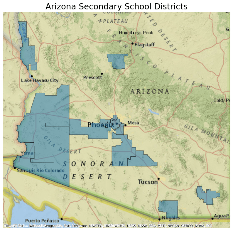
The map created shows the Arizona Secondary School Districts.
School Districts - Unified (UNSD)
This file contains Unified School Districts, referring to districts that provide education to children of all school ages. Unified school districts can have both secondary and elementary schools.
The attribute table contains the following information:
- STATEFP = State FIPS code
- UNSDLEA = Unified School District local education agency code
- AFFGEOID = American FactFinder summary level code + geovariant code + "00US" + GEOID
- GEOID = Concatenation of State FIPS code and UNSDLEA code
- NAME = Unified School District name
- STUSPS = FIPS Postal code
- STATE_NAME = State name
- LSAD = Legal/statistical classification
- ALAND = Current land area
- AWATER = Current water area
- geometry = Coordinates for Unified School District polygons
Use the read_parquet function of Dask-GeoPandas to read the Unified School Districts data from the parquet file of the Planetary Computer dataset:
asset = census.get_item("2020-cb_2020_us_unsd_500k").assets["data"]
ddf = geopandas.read_parquet(
    asset.href, storage_options=asset.extra_fields["table:storage_options"]
)
ddf.head()
| STATEFP | UNSDLEA | AFFGEOID | GEOID | NAME | STUSPS | STATE_NAME | LSAD | ALAND | AWATER | geometry | |
|---|---|---|---|---|---|---|---|---|---|---|---|
| 0 | 36 | 18210 | 9700000US3618210 | 3618210 | Malverne Union Free School District | NY | New York | 00 | 5271104 | 539214 | POLYGON ((-73.67603 40.67130, -73.67428 40.672... |
| 1 | 29 | 21660 | 9700000US2921660 | 2921660 | Northeast Nodaway County R-V School District | MO | Missouri | 00 | 292199326 | 69164 | POLYGON ((-94.78484 40.37451, -94.77798 40.373... |
| 2 | 29 | 9930 | 9700000US2909930 | 2909930 | Blair Oaks R-II School District | MO | Missouri | 00 | 181982856 | 5337193 | POLYGON ((-92.25955 38.37702, -92.25574 38.381... |
| 3 | 29 | 11550 | 9700000US2911550 | 2911550 | Cole County R-V School District | MO | Missouri | 00 | 368295288 | 3182437 | POLYGON ((-92.46801 38.31442, -92.46697 38.327... |
| 4 | 51 | 2490 | 9700000US5102490 | 5102490 | Middlesex County Public Schools | VA | Virginia | 00 | 337554148 | 208310589 | MULTIPOLYGON (((-76.42081 37.59787, -76.41957 ... |
Next, plot the data from this parquet file and overlay it on a basemap. For this example, select the entire New York City Unified School District, which encompasses the five counties of NYC. Select the relevant data by filtering by the NAME column.
ddf.crs = 4326
ddf = ddf.to_crs(epsg=3857)

ax = ddf[ddf.NAME == "New York City Department Of Education"].plot(
    figsize=(10, 10), alpha=0.5, edgecolor="k"
)
ax.set_title(
    "New York City Unified School District",
    fontdict={"fontsize": "20", "fontweight": "2"},
)
ctx.add_basemap(ax, source=ctx.providers.Esri.NatGeoWorldMap)
ax.set_axis_off()
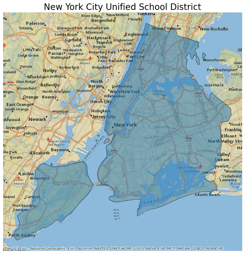
The map created shows the New York City Unified School District.
State Legislative Districts
State Legislative Districts is the fourth grouping of datasets within the census data by cartographic boundaries group. This dataset grouping includes State Legislative Districts for both Upper and Lower State Chambers. These are areas in which voters elect a person to represent them in state or equivalent entity legislatures. Most states have both upper and lower chambers, the exceptions being Nebraska which has a unicameral legislature, and Washington, DC, which has a single council. As a result, there is no lower house data for Nebraska and DC.
State Legislative Districts - Lower Chamber (SLDL)
This file contains Lower Chamber State Legislative Districts.
The attribute table contains the following information:
- STATEFP = State FIPS code
- SLDLST = State Legislative District Lower Chamber code
- AFFGEOID = American FactFinder summary level code + geovariant code + "00US" + GEOID
- GEOID = Concatenation of State FIPS code and SLDLST
- NAME = District Name
- NAMELSAD = District name and legal/statistical description
- STUSPS = FIPS Postal code
- STATE_NAME = State name
- LSAD = Legal/statistical classification
- LSY = Legislative Session Year
- ALAND = Current land area
- AWATER = Current water area
- geometry = coordinates for Lower Chamber polygons
Use the read_parquet function of Dask-GeoPandas to read the Lower Chamber State Legislative Districts data from the parquet file of the Planetary Computer dataset:
asset = census.get_item("2020-cb_2020_us_sldl_500k").assets["data"]
ddf = geopandas.read_parquet(
    asset.href, storage_options=asset.extra_fields["table:storage_options"]
)
ddf.head()
| STATEFP | SLDLST | AFFGEOID | GEOID | NAME | NAMELSAD | STUSPS | STATE_NAME | LSAD | LSY | ALAND | AWATER | geometry | |
|---|---|---|---|---|---|---|---|---|---|---|---|---|---|
| 0 | 37 | 067 | 620L600US37067 | 37067 | 67 | State House District 67 | NC | North Carolina | LL | 2018 | 1372481845 | 13054913 | POLYGON ((-80.67249 35.28457, -80.66859 35.284... |
| 1 | 37 | 023 | 620L600US37023 | 37023 | 23 | State House District 23 | NC | North Carolina | LL | 2018 | 2498112701 | 4460107 | POLYGON ((-77.82844 35.86721, -77.82613 35.871... |
| 2 | 39 | 078 | 620L600US39078 | 39078 | 78 | State House District 78 | OH | Ohio | LL | 2018 | 3609975942 | 28657516 | POLYGON ((-83.01738 39.73643, -83.01428 39.738... |
| 3 | 41 | 026 | 620L600US41026 | 41026 | 26 | State House District 26 | OR | Oregon | LL | 2018 | 209051898 | 1046849 | POLYGON ((-122.95072 45.44942, -122.94726 45.4... |
| 4 | 41 | 015 | 620L600US41015 | 41015 | 15 | State House District 15 | OR | Oregon | LL | 2018 | 517343089 | 8286102 | POLYGON ((-123.26079 44.55749, -123.26025 44.5... |
Next, plot the data from this parquet file and overlay it on a basemap. For this example, plot all the Lower Chamber State Legislative Districts in Texas by filtering by "TX" in the STUSPS column.
ddf.crs = 4326
ddf = ddf.to_crs(epsg=3857)

ax = ddf[ddf.STUSPS == "TX"].plot(figsize=(10, 10), alpha=0.5, edgecolor="k")
ax.set_title(
    "State Legislative Districts: Texas, Lower Chamber",
    fontdict={"fontsize": "20", "fontweight": "2"},
)
ctx.add_basemap(ax, source=ctx.providers.Esri.NatGeoWorldMap)
ax.set_axis_off()
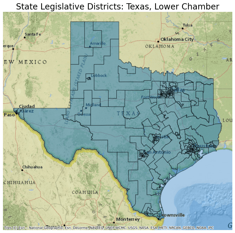
The map created shows the Texas Lower Chamber State Legislative Districts.
State Legislative Districts - Upper Chamber (SLDU)
This file contains Upper Chamber State Legislative Districts.
The attribute table contains the following information:
- STATEFP = State FIPS code
- SLDUST = State Legislative District Upper Chamber code
- AFFGEOID = American FactFinder summary level code + geovariant code + "00US" + GEOID
- GEOID = Concatenation of State FIPS code and SLDUST
- NAME = District Name
- NAMELSAD = District name and legal/statistical description
- STUSPS = FIPS Postal code
- STATE_NAME = State name
- LSAD = Legal/statistical classification
- LSY = Legislative Session Year
- ALAND = Current land area
- AWATER = Current water area
- geometry = coordinates for Upper Chamber polygon
Use the read_parquet function of Dask-GeoPandas to read the Upper Chamber State Legislative Districts data from the parquet file of the Planetary Computer dataset:
asset = census.get_item("2020-cb_2020_us_sldu_500k").assets["data"]
ddf = geopandas.read_parquet(
    asset.href, storage_options=asset.extra_fields["table:storage_options"]
)
ddf.head()
| STATEFP | SLDUST | AFFGEOID | GEOID | NAME | NAMELSAD | STUSPS | STATE_NAME | LSAD | LSY | ALAND | AWATER | geometry | |
|---|---|---|---|---|---|---|---|---|---|---|---|---|---|
| 0 | 41 | 004 | 610U600US41004 | 41004 | 4 | State Senate District 4 | OR | Oregon | LU | 2018 | 16139528745 | 167874360 | POLYGON ((-123.81715 43.45959, -123.81666 43.5... |
| 1 | 41 | 015 | 610U600US41015 | 41015 | 15 | State Senate District 15 | OR | Oregon | LU | 2018 | 238454422 | 423501 | POLYGON ((-123.15350 45.53457, -123.15271 45.5... |
| 2 | 42 | 016 | 610U600US42016 | 42016 | 16 | State Senate District 16 | PA | Pennsylvania | LU | 2018 | 796458250 | 5947856 | POLYGON ((-75.88921 40.67834, -75.85481 40.693... |
| 3 | 48 | 015 | 610U600US48015 | 48015 | 15 | State Senate District 15 | TX | Texas | LU | 2018 | 828734514 | 37403360 | POLYGON ((-95.57473 29.86719, -95.56919 29.867... |
| 4 | 51 | 016 | 610U600US51016 | 51016 | 16 | State Senate District 16 | VA | Virginia | LU | 2018 | 580535957 | 32576935 | POLYGON ((-77.59806 37.23679, -77.59600 37.238... |
Next, plot the data from this parquet file and overlay it on a basemap. For this example, plot all the Upper Chamber State Legislative Districts in Michigan by filtering by "MI" in the STUSPS column.
ddf.crs = 4326
ddf = ddf.to_crs(epsg=3857)

ax = ddf[ddf.STUSPS == "MI"].plot(figsize=(10, 10), alpha=0.5, edgecolor="k")
ax.set_title(
    "State Legislative Districts: Michigan, Upper Chamber",
    fontdict={"fontsize": "20", "fontweight": "2"},
)
ctx.add_basemap(ax, source=ctx.providers.Esri.NatGeoWorldMap)
ax.set_axis_off()
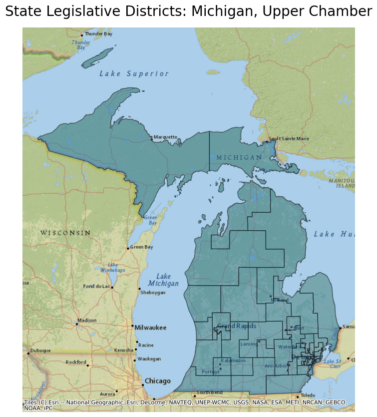
The map created shows the Michigan Upper Chamber State Legislative Districts.
States (STATE)
This file contains the US States and State Equivalent Entities. Within Census Bureau datasets, the District of Columbia, Puerto Rico, and the Island Areas (American Samoa, the Commonwealth of the Northern Mariana Islands, Guam, and the US Virgin Islands) are treated as statistical equivalents of states alongside the 50 US states.
The attribute table contains the following information:
- STATEFP = State FIPS code
- STATENS = State ANSI feature code
- AFFGEOID = American FactFinder summary level code + geovariant code + "00US" + GEOID
- GEOID = STATEFP
- STUSPS = FIPS postal code
- NAME = State name
- LSAD = Legal/statistical classification
- ALAND = Current land area
- AWATER = Current water area
- geometry = coordinates for State polygons
Use the read_parquet function of Dask-GeoPandas to read the US States and State Equivalent Entities data from the parquet file of the Planetary Computer dataset:
asset = census.get_item("2020-cb_2020_us_state_500k").assets["data"]
ddf = geopandas.read_parquet(
    asset.href, storage_options=asset.extra_fields["table:storage_options"]
)
ddf.head()
| STATEFP | STATENS | AFFGEOID | GEOID | STUSPS | NAME | LSAD | ALAND | AWATER | geometry | |
|---|---|---|---|---|---|---|---|---|---|---|
| 0 | 66 | 1802705 | 0400000US66 | 66 | GU | Guam | 00 | 543555847 | 934337453 | MULTIPOLYGON (((144.64538 13.23627, 144.64716 ... |
| 1 | 48 | 1779801 | 0400000US48 | 48 | TX | Texas | 00 | 676680588914 | 18979352230 | MULTIPOLYGON (((-94.71830 29.72885, -94.71721 ... |
| 2 | 55 | 1779806 | 0400000US55 | 55 | WI | Wisconsin | 00 | 140292246684 | 29343721650 | MULTIPOLYGON (((-86.95617 45.35549, -86.95463 ... |
| 3 | 44 | 1219835 | 0400000US44 | 44 | RI | Rhode Island | 00 | 2677759219 | 1323691129 | MULTIPOLYGON (((-71.28802 41.64558, -71.28647 ... |
| 4 | 36 | 1779796 | 0400000US36 | 36 | NY | New York | 00 | 122049520861 | 19256750161 | MULTIPOLYGON (((-72.03683 41.24984, -72.03496 ... |
Next, plot the data from this parquet file and overlay it on a basemap. For this example, plot only the contiguous US, Puerto Rico, and the US Virgin Islands. To exclude parts of the dataset from plotting, use ~df.STATEFP.isin() to exclude the STATEFP codes for Alaska, Hawaii, Guam, American Samoa, and the Commonwealth of the Northern Mariana Islands.
ddf.crs = 4326
ddf = ddf.to_crs(epsg=3857)

ax = ddf[~ddf.STATEFP.isin(["02", "15", "60", "66", "69"])].plot(
    figsize=(10, 10), alpha=0.5, edgecolor="k"
)
ax.set_title(
    "States: Contiguous US, Puerto Rico, & USVI",
    fontdict={"fontsize": "20", "fontweight": "2"},
)
ctx.add_basemap(ax, source=ctx.providers.Esri.NatGeoWorldMap)
ax.set_axis_off()
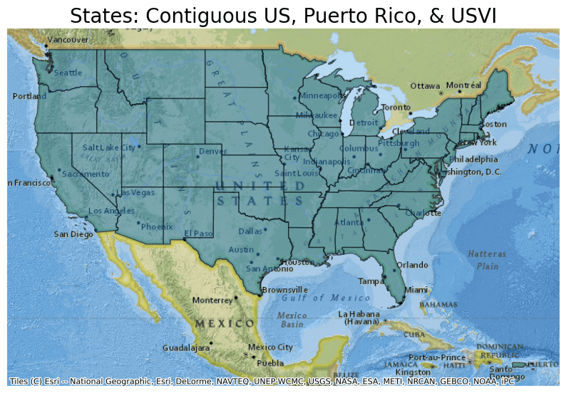
The map created shows the Contiguous US, Puerto Rico, and the US Virgin Islands.
Subbarrios (SUBBARRIO)
This file contains Subbarrios, which are legally defined subdivisions of Minor Civil Division in Puerto Rico. They don"t exist within every Minor Civil Division and don"t always cover the entire Minor Civil Division where they do exist.
The attribute table contains the following information:
- STATEFP = State FIPS code
- COUNTYFP = County FIPS code
- COUSUBFP = County Subdivision FIPS code
- SUBMCDFP = Subbarrio FIPS code
- SUBMCDNS = Subbarrio ANSI feature code
- AFFGEOID = American FactFinder summary level code + geovariant code + "00US" + GEOID
- GEOID = Concatenation of State FIPS code, County FIPS code, County Subdivision FIPS code and Subbarrio FIPS code
- NAME = Subbarrio name
- NAMELSAD = Subbarrio name and legal/statistical division
- LSAD = Legal/statistical classification
- ALAND = Current land area
- AWATER = Current water area
- geometry = coordinates for Subbarrio polygons
Use the read_parquet function of Dask-GeoPandas to read the Subbarrios data from the parquet file of the Planetary Computer dataset:
asset = census.get_item("2020-cb_2020_72_subbarrio_500k").assets["data"]
ddf = geopandas.read_parquet(
    asset.href, storage_options=asset.extra_fields["table:storage_options"]
)
ddf.head()
| STATEFP | COUNTYFP | COUSUBFP | SUBMCDFP | SUBMCDNS | AFFGEOID | GEOID | NAME | NAMELSAD | LSAD | ALAND | AWATER | geometry | |
|---|---|---|---|---|---|---|---|---|---|---|---|---|---|
| 0 | 72 | 035 | 15537 | 65040 | 2415842 | 0670000US720351553765040 | 720351553765040 | Pueblo Sur | Pueblo Sur subbarrio | 51 | 2708525 | 517 | POLYGON ((-66.18201 18.11012, -66.18182 18.110... |
| 1 | 72 | 127 | 84079 | 84771 | 2416087 | 0670000US721278407984771 | 721278407984771 | Valencia | Valencia subbarrio | 51 | 144073 | 0 | POLYGON ((-66.04345 18.41148, -66.04334 18.411... |
| 2 | 72 | 127 | 79693 | 34770 | 2415499 | 0670000US721277969334770 | 721277969334770 | Hipódromo | Hipódromo subbarrio | 51 | 263788 | 0 | POLYGON ((-66.07415 18.44463, -66.07115 18.448... |
| 3 | 72 | 013 | 03411 | 72325 | 2415953 | 0670000US720130341172325 | 720130341172325 | Rosario | Rosario subbarrio | 51 | 58332 | 12520 | POLYGON ((-66.71531 18.47233, -66.71231 18.472... |
| 4 | 72 | 121 | 73587 | 64805 | 2415826 | 0670000US721217358764805 | 721217358764805 | Pueblo Norte | Pueblo Norte subbarrio | 51 | 120549 | 0 | POLYGON ((-66.96232 18.07969, -66.96186 18.080... |
Next, plot the data from this parquet file and overlay it on a basemap. For this example, plot all the Subbarrios in the San Juan Municipo (the county equivalent for Puerto Rico). Select the relevant data by filtering by the COUNTYFP column.
ddf.crs = 4326
ddf = ddf.to_crs(epsg=3857)

ax = ddf[ddf.COUNTYFP == "127"].plot(figsize=(10, 10), alpha=0.5, edgecolor="k")
ax.set_title(
    "Subbarrios: San Juan, Puerto Rico",
    fontdict={"fontsize": "20", "fontweight": "2"},
)
ctx.add_basemap(ax, source=ctx.providers.Esri.NatGeoWorldMap)
ax.set_axis_off()
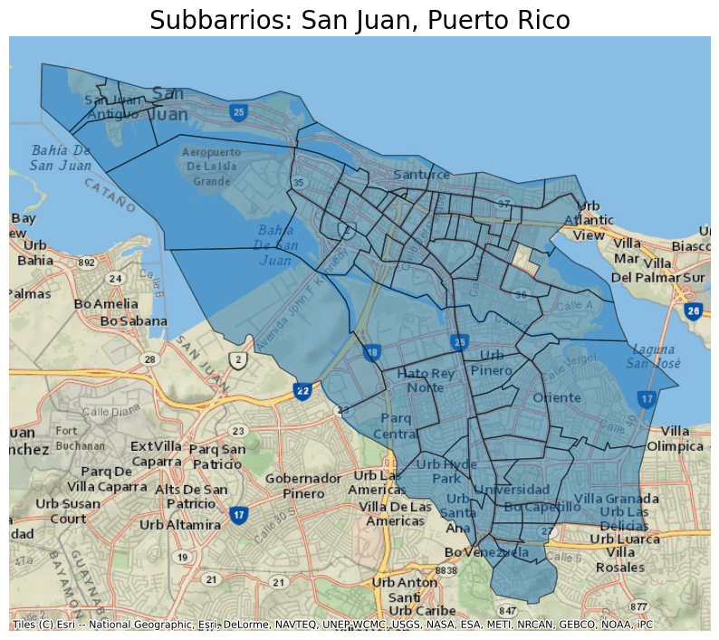
The map created shows the Subbarrios in San Juan Municipo.
United States Outline
This file contains the United States Outline shapefile. This contains all 50 US states plus the District of Columbia, Puerto Rico, and the Island Areas (American Samoa, the Commonwealth of the Northern Mariana Islands, Guam, and the US Virgin Islands). There is only one feature within this dataset.
The attribute table for this dataset only contains the AFFGEOID, GEOID, NAME, and coordinates for the US polygon.
Use the read_parquet function of Dask-GeoPandas to read the United States Outline data from the parquet file of the Planetary Computer dataset:
asset = census.get_item("2020-cb_2020_us_nation_5m").assets["data"]
ddf = geopandas.read_parquet(
    asset.href, storage_options=asset.extra_fields["table:storage_options"]
)
ddf.head()
| AFFGEOID | GEOID | NAME | geometry | |
|---|---|---|---|---|
| 0 | 0100000US | US | United States | MULTIPOLYGON (((179.48246 51.98283, 179.48656 ... |
Next, plot the entire data from this parquet file and overlay it on a basemap. Since this dataset contains only one feature, there are no options to select or exclude specific parts based on attributes.
ddf.crs = 4326
ddf = ddf.to_crs(epsg=3857)

ax = ddf.plot(figsize=(30, 60), alpha=0.5, edgecolor="k")
ax.set_title(
    "United States and US Overseas Territories",
    fontdict={"fontsize": "20", "fontweight": "2"},
)
ctx.add_basemap(ax, source=ctx.providers.Esri.NatGeoWorldMap)
ax.set_axis_off()
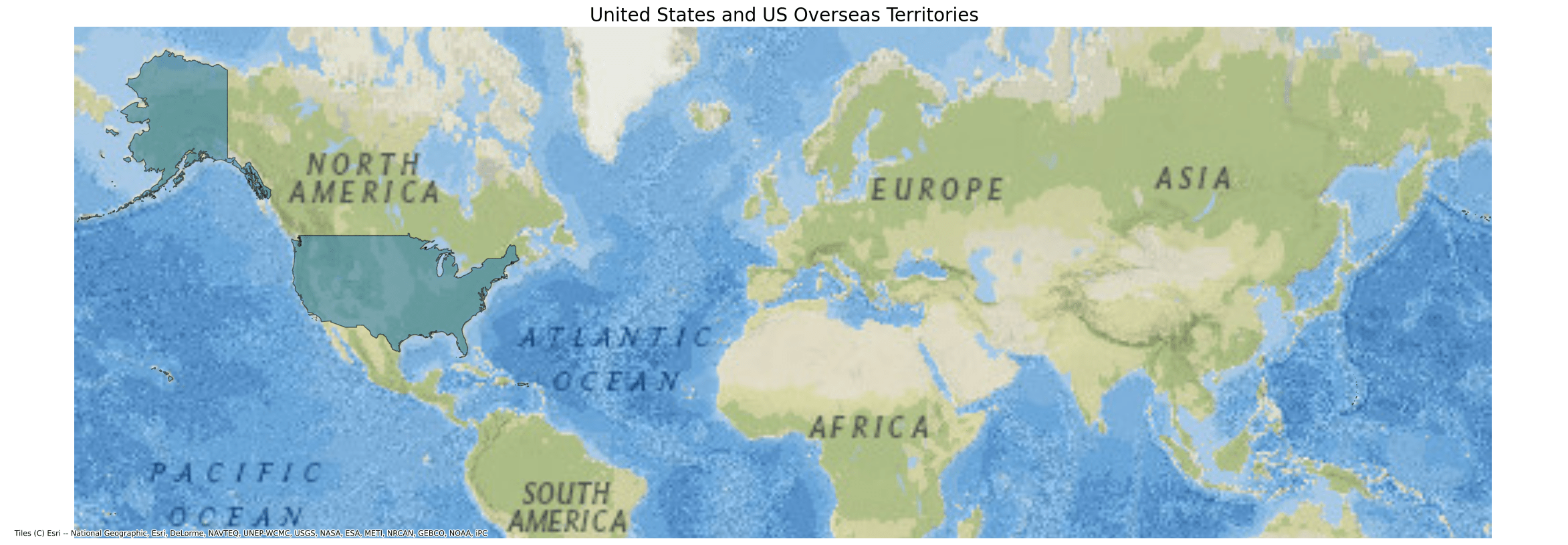
The map created shows the United States and US Overseas Territories.
Voting Districts (VTD)
This file contains all US Voting Districts, which are geographic features established by state, local and tribal governments to conduct elections.
The attribute table contains the following information:
- STATEFP20 = State FIPS code
- COUNTYFP20 = County FIPS code
- VTDST20 = Voting district code
- AFFGEOID = American FactFinder summary level code + geovariant code + "00US" + GEOID
- EOID = Concatenation of State FIPS code, County FIPS code, and Voting District code
- VTDI20 = Voting district indicator
- NAME20 = Voting district name
- NAMELSAD20 = Voting district name and legal/statistical division
- LSAD20 = Legal/statistical classification
- ALAND20 = Current land area
- AWATER20 = Current water area
- geometry = coordinates for Voting District polygons
Use the read_parquet function of Dask-GeoPandas to read the Voting Districts data from the parquet file of the Planetary Computer dataset:
asset = census.get_item("2020-cb_2020_us_vtd_500k").assets["data"]
ddf = geopandas.read_parquet(
    asset.href, storage_options=asset.extra_fields["table:storage_options"]
)
ddf.head()
| STATEFP20 | COUNTYFP20 | VTDST20 | AFFGEOID20 | GEOID20 | VTDI20 | NAME20 | NAMELSAD20 | LSAD20 | ALAND20 | AWATER20 | geometry | |
|---|---|---|---|---|---|---|---|---|---|---|---|---|
| 0 | 24 | 003 | 06-024 | 7000000US2400306-024 | 2400306-024 | A | ANNE ARUNDEL PRECINCT 06-024 | ANNE ARUNDEL PRECINCT 06-024 | 00 | 2756767 | 21979454 | POLYGON ((-76.48621 38.92784, -76.48142 38.928... |
| 1 | 24 | 047 | 01-002 | 7000000US2404701-002 | 2404701-002 | A | WORCESTER PRECINCT 01-002 | WORCESTER PRECINCT 01-002 | 00 | 111861087 | 1934368 | MULTIPOLYGON (((-75.30048 38.09594, -75.29902 ... |
| 2 | 02 | 090 | 06-150 | 7000000US0209006-150 | 0209006-150 | A | Fox Precinct | Fox Precinct | 00 | 2241567797 | 0 | POLYGON ((-148.11011 65.20532, -148.10451 65.2... |
| 3 | 26 | 101 | 101001 | 7000000US26101101001 | 26101101001 | A | 1010332000001 | Voting District 1010332000001 | V1 | 48159260 | 1006220 | POLYGON ((-86.25160 44.46544, -86.25091 44.469... |
| 4 | 26 | 055 | 055007 | 7000000US26055055007 | 26055055007 | A | 0552380000001 | Voting District 0552380000001 | V1 | 9967698 | 0 | POLYGON ((-85.57537 44.75340, -85.57330 44.752... |
Next, plot the data from this parquet file and overlay it on a basemap. For this example, plot all the Voting Districts in Salt Lake City, UT by filtering by Voting District Names that begin with "Salt Lake" in the NAME20 column.
ddf.crs = 4326
ddf = ddf.to_crs(epsg=3857)

ax = ddf[ddf.NAME20.str.startswith("Salt Lake")].plot(
    figsize=(10, 10), alpha=0.5, edgecolor="k"
)
ax.set_title(
    "Salt Lake City Voting Districts",
    fontdict={"fontsize": "20", "fontweight": "2"},
)
ctx.add_basemap(ax, source=ctx.providers.Esri.NatGeoWorldMap)
ax.set_axis_off()
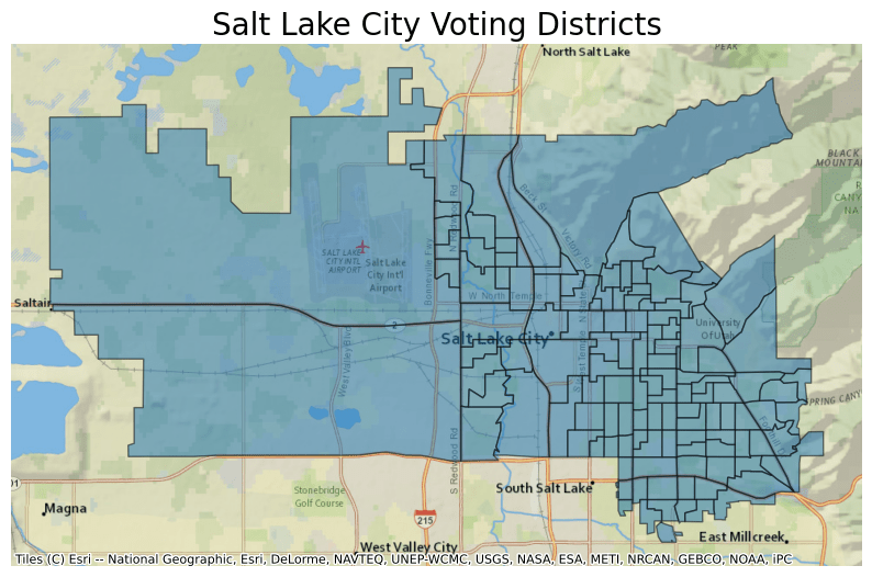
The map created shows Salt Lake City Voting Districts.