Reprojecting and Resampling¶

In this tutorial, you'll learn how to reproject Cloud Optimized GeoTIFFs (COG) into a different Coordinate Reference System (CRS). Reprojecting data usually also includes resampling the raster data to a different resolution, which requires combining multiple pixel values into (when downsampling -- or resampling to lower resolution/larger cellsizes) or interpolating new pixels from the existing ones (when upsampling -- or resampling to higher resolution/smaller cellsizes). You will also learn how to use different resampling algorithms to adjust the raster pixel size.

This tutorial covers several methods for reprojecting. Which one to pick depends primarily on two factors:

whether you already know what CRS you are targeting when you load your data
whether you have STAC Items for the data you're working with

In general, reprojecting and resampling while loading the data is more efficient, and all the remote-sensing datasets in the Planetary Computer's data catalog include STAC Items.

This tutorial covers the following four methods for reprojecting and resampling geodata:

Method 1: Reproject and resample a large number of COGs *while loading* using stackstac. This method requires STAC items.
Method 2: Reproject and resample a single COG *while loading* with rioxarray and rasterio using a WarpedVRT. This option works without STAC items but won't scale to a large number of COGs.
Method 3: Reproject and resample an in-memory (potentially distributed) DataArray with stackstac.reproject_array. This option requires more memory and is generally less efficient than option 1, but you don't need to know the destination CRS when loading your data.
Method 4: Reproject and resample an in-memory (single machine) DataArray using rioxarray and rasterio. This option only works on a single machine and requires more memory than option 2, but you don't need to know the destination CRS when loading your data.

These reprojection methods are ranked in order of what is generally recommended. However, certain methods may not be available depending on whether you know your destination CRS while loading the data and whether you have STAC Items.

In [1]:

import planetary_computer
import pystac_client

import numpy as np
import xarray as xr

import stackstac
import affine
import pyproj
import rioxarray
import rasterio

from rioxarray.rioxarray import _make_coords
from rasterio.vrt import WarpedVRT

import xrspatial.multispectral as ms
import matplotlib.pyplot as plt

Preparation: Create a local Dask cluster¶

In this tutorial, you'll be using a small dataset. Create a local Dask cluster to process the data in parallel using all the cores of your machine.

In [2]:

from dask.distributed import Client

client = Client()
print(f"/proxy/{client.scheduler_info()['services']['dashboard']}/status")

2022-08-16 16:36:43,441 - distributed.diskutils - INFO - Found stale lock file and directory '/tmp/dask-worker-space/worker-iajxxwmr', purging
2022-08-16 16:36:43,442 - distributed.diskutils - INFO - Found stale lock file and directory '/tmp/dask-worker-space/worker-0_6rl8kn', purging
2022-08-16 16:36:43,442 - distributed.diskutils - INFO - Found stale lock file and directory '/tmp/dask-worker-space/worker-rml0ni71', purging
2022-08-16 16:36:43,442 - distributed.diskutils - INFO - Found stale lock file and directory '/tmp/dask-worker-space/worker-9lcurr39', purging

/proxy/8787/status

To follow the progress of your computation, you can access the Dask Dashboard at the URL from the previous cell's output.

The region of interest for this tutorial is located in Colorado, USA, centered by Cochetopa Dome and Sawtooth Mountain. You'll be using Sentinel-2 Level-2A data. See Reading data from the STAC API for more information on accessing data through the STAC API.

In [3]:

stac = pystac_client.Client.open(
    "https://planetarycomputer.microsoft.com/api/stac/v1/",
    modifier=planetary_computer.sign_inplace,
)
search = stac.search(
    collections=["sentinel-2-l2a"],
    intersects={"type": "Point", "coordinates": [-106.714900, 38.22679]},
    query={"eo:cloud_cover": {"lt": 1}},
    datetime="2019-09-01/2019-09-30",
)

item = next(search.items())

Method 1: Reproject and resample while loading with stackstac.stack ¶

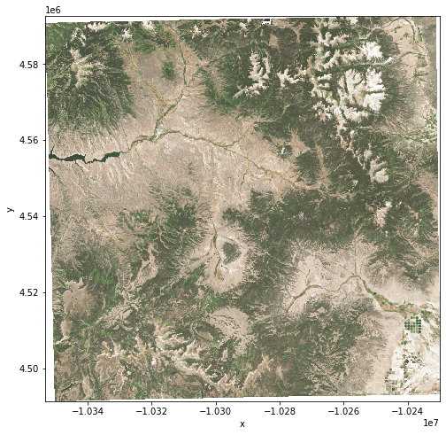
The selected scene is stored in an EPSG:32613 coordinate system. Let's reproject it to a new CRS by providing the destination epsg number to the stackstac.stack function. To adjust the data's resolution, also provide values to the function's optional resolution and resampling parameters.

With stackstac.stack, you can use any CRS as defined by an EPSG code. In this example, you use the stackstac.stack function to reproject to the Lambert Cylindrical projection (epsg:6933). Lambert Cylindrical is an equal-area projection that preserves area measurements. Regions with the same size on the Earth's surface have the same size on the map. However, shapes, angles, and scales are generally distorted.

This example uses the bilinear resampling method. Resampling happens in the stackstac.stack function as well. As this function uses rasterio internally, you can use any algorithm from the rasterio.enums.Resampling class. To use a specific algorithm, pass it as a value for the resampling parameter. The default resampling method in stackstac.stack is rasterio.enums.Resampling.nearest.

In [4]:

scene_data = (
    stackstac.stack(
        [item.to_dict()],
        epsg=6933,
        resampling=rasterio.enums.Resampling.bilinear,
        resolution=100,  # resolution in the output CRS’s units
        assets=["B04", "B03", "B02"],  # red, green, blue bands
        chunksize=2048,
    )
    .isel(time=0)
    .persist()
)

scene_data

Out[4]:

<xarray.DataArray 'stackstac-22268e1e94fdf2bbacd6eb69e3399611' (band: 3,
                                                                y: 1013, x: 1235)>
dask.array<getitem, shape=(3, 1013, 1235), dtype=float64, chunksize=(1, 1013, 1235), chunktype=numpy.ndarray>
Coordinates: (12/46)
    time                                     datetime64[ns] 2019-09-24T17:50:...
    id                                       <U54 'S2B_MSIL2A_20190924T175049...
  * band                                     (band) <U3 'B04' 'B03' 'B02'
  * x                                        (x) float64 -1.035e+07 ... -1.02...
  * y                                        (y) float64 4.593e+06 ... 4.491e+06
    s2:saturated_defective_pixel_percentage  float64 0.0
    ...                                       ...
    proj:transform                           object {0.0, 300000.0, 10.0, 430...
    proj:shape                               object {10980}
    common_name                              (band) <U5 'red' 'green' 'blue'
    center_wavelength                        (band) float64 0.665 0.56 0.49
    full_width_half_max                      (band) float64 0.038 0.045 0.098
    epsg                                     int64 6933
Attributes:
    spec:        RasterSpec(epsg=6933, bounds=(-10353400, 4491300, -10229900,...
    crs:         epsg:6933
    transform:   | 100.00, 0.00,-10353400.00|\n| 0.00,-100.00, 4592600.00|\n|...
    resolution:  100

To generate a preview of the reprojected and resampled data, create a true color image with the xrspatil.multispectral.true_color function.

Provide the following parameters:

the three bands of red, green, blue in your scene_data
the optional string value name for the image's name

Note: To adjust contrast and brightness, provide values for the two optional numeric parameters c (contrast) and th (brightness). All image previews in this tutorial use the function's default values of c=10 and th=0.125.

In [5]:

# visualize selected scene
cylindrical_img = ms.true_color(*scene_data, name="epsg=6933")
cylindrical_img.plot.imshow(figsize=(8, 8));

Method 2: Reproject and resample while loading with rasterio and rioxarray using a `WarpedVRT`¶

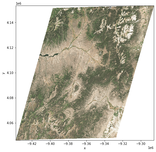
The STAC item we selected has various assets, one per band, which link to COGs in Azure Blob Storage. This example will reproject and resample those bands from their source CRS of EPSG:32613 to the Robinson CRS of ESRI:54030. The Robinson projection aims to show the entire globe at once and is neither equal-area nor conformal.

With rasterio's WarpedVRT class, you only need to provide the geodata's URL as input parameters. You don't need to download any GeoTIFF files beforehand. Resampling works similar to method 1 above: you can specify the resampling method as one of the algorithms available in rasterio.enums.Resampling. If you don't provide a resampling method, rasterio will use the default option of rasterio.enums.Resampling.nearest. Let's use the average resampling method in this example.

In [6]:

urls = {
    "red": item.assets["B04"].href,
    "green": item.assets["B03"].href,
    "blue": item.assets["B02"].href,
}

The Robinson projection is a map projection that does not preserve equal-area nor conformality. As a compromise, both the altitude and longitude lines are evenly spaced across the map.

Follow these steps to reproject and resample your data from EPSG:32613 to the Robinson CRS of ESRI:54030:

Step 1: Get the rasterio CRS for ESRI:54030.

In [7]:

robinson_crs = pyproj.crs.CRS.from_string("ESRI:54030")
robinson_crs = rasterio.crs.CRS.from_wkt(robinson_crs.to_wkt())
robinson_crs

Out[7]:

CRS.from_wkt('PROJCS["World_Robinson",GEOGCS["WGS 84",DATUM["WGS_1984",SPHEROID["WGS 84",6378137,298.257223563]],PRIMEM["Greenwich",0],UNIT["Degree",0.0174532925199433]],PROJECTION["Robinson"],PARAMETER["longitude_of_center",0],PARAMETER["false_easting",0],PARAMETER["false_northing",0],UNIT["metre",1],AXIS["Easting",EAST],AXIS["Northing",NORTH],AUTHORITY["ESRI","54030"]]')

Note that in case you want to reproject to an EPSG CRS (such as EPSG:4326), you have the option to use only the number (such as 4326) as the destination CRS.

Step 2: Define a shape (height, width) and bounding box (coordinates) for the reprojected destination image.

In [8]:

height = width = 1000
robinson_bounds = (-9438051, 4153437, -9285636, 4046189)

Step 3: Calculate a transform to reproject from the source CRS to the destination CRS and resolution.

In [9]:

left, bottom, right, top = robinson_bounds
xres = (right - left) / width
yres = (top - bottom) / height
robinson_transform = affine.Affine(xres, 0.0, left, 0.0, -yres, top)

robinson_transform

Out[9]:

Affine(152.415, 0.0, -9438051.0,
       0.0, 107.248, 4046189.0)

Step 4: Provide all information to WarpedVRT (destination CRS, destination transform, destination shape, and resampling method).

In [10]:

robinson_vrt_options = {
    "crs": robinson_crs,
    "transform": robinson_transform,
    "height": height,
    "width": width,
    "resampling": rasterio.enums.Resampling.average,
}

robinson_reproj = []

for _, url in urls.items():
    with rasterio.open(url) as src:
        with WarpedVRT(src, **robinson_vrt_options) as vrt:
            reproj = rioxarray.open_rasterio(vrt).chunk(
                {"x": 1000, "y": 1000, "band": 1}
            )
            robinson_reproj.append(reproj)

robinson_reproj = xr.concat(robinson_reproj, dim="band")

Step 5: Visualize the projection.

In [11]:

robinson_img = ms.true_color(*robinson_reproj, name="esri=54030")
robinson_img.plot.imshow(figsize=(8, 8));

Method 3: Reproject and resample an in-memory array with stackstac.reproject_array ¶

stackstac.reproject_array will reproject and clip an xarray.DatArray using scipy.interpolate.interpn internally. To specify the resampling method, set the optional interpolation parameter to one of the two available interpolation methods: linear or nearest (default).

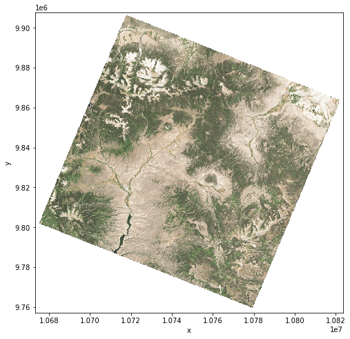
This example uses the Space Oblique projection (EPSG: 29873). This projection was explicitly created for satellite imagery and is designed to be free of distortion along the orbit path of a satellite. For resampling, this example uses linear interpolation with a target resolution of (100, 100).

Step 1: Use the stackstac.array_bounds function to get the bounds of your input data in the target CRS. The input data for this example is the DataArray called scene_data you created for the first method described in this notebook.

In [12]:

space_oblique_crs = 29873
space_oblique_bounds = stackstac.array_bounds(scene_data, space_oblique_crs)

space_oblique_bounds

Out[12]:

(10673196.491207449, 9757187.12410703, 10823668.536491105, 9907712.523330946)

Step 2: Create a RasterSpec object with the target CRS, the bounds from the previous step, and the target resolution.

In [13]:

space_oblique_resolution = (100, 100)
space_oblique_spec = stackstac.raster_spec.RasterSpec(
    epsg=space_oblique_crs,
    bounds=space_oblique_bounds,
    resolutions_xy=space_oblique_resolution,
)

space_oblique_spec

Out[13]:

RasterSpec(epsg=29873, bounds=(10673196.491207449, 9757187.12410703, 10823668.536491105, 9907712.523330946), resolutions_xy=(100, 100))

Step 3: Reproject and resample the data with reproject_array, using the DataArray scene_data and the RasterSpec from the previous step. This is also where you define the resampling method to be "linear".

In [14]:

space_oblique_reproj = stackstac.reproject_array(
    arr=scene_data,
    spec=space_oblique_spec,
    interpolation="linear",
)

space_oblique_reproj

Out[14]:

<xarray.DataArray 'stackstac-22268e1e94fdf2bbacd6eb69e3399611' (band: 3,
                                                                y: 1505, x: 1505)>
dask.array<dask_aware_interpnd, shape=(3, 1505, 1505), dtype=float64, chunksize=(1, 1505, 1505), chunktype=numpy.ndarray>
Coordinates: (12/48)
    time                                     datetime64[ns] 2019-09-24T17:50:...
    id                                       <U54 'S2B_MSIL2A_20190924T175049...
  * band                                     (band) <U3 'B04' 'B03' 'B02'
    s2:saturated_defective_pixel_percentage  float64 0.0
    s2:degraded_msi_data_percentage          float64 0.0
    s2:water_percentage                      float64 0.2779
    ...                                       ...
    full_width_half_max                      (band) float64 0.038 0.045 0.098
    epsg                                     int64 6933
    x_6933                                   (y, x) float64 -1.025e+07 ... -1...
    y_6933                                   (y, x) float64 4.629e+06 ... 4.4...
  * y                                        (y) float64 9.908e+06 ... 9.757e+06
  * x                                        (x) float64 1.067e+07 ... 1.082e+07
Attributes:
    spec:        RasterSpec(epsg=6933, bounds=(-10353400, 4491300, -10229900,...
    crs:         epsg:6933
    transform:   | 100.00, 0.00,-10353400.00|\n| 0.00,-100.00, 4592600.00|\n|...
    resolution:  100

Step 4: Visualize the projection.

In [15]:

space_oblique_img = ms.true_color(*space_oblique_reproj, name="epsg=29873")
space_oblique_img.plot.imshow(figsize=(8, 8));

Method 4: Reproject and resample an in-memory DataArray with rasterio and rioxarray ¶

Rasterio and rioxarray both provide tools for raster warping and reprojection. They both use GDAL under the hood.

Reproject and resample in-memory data with rasterio's `reproject()`¶

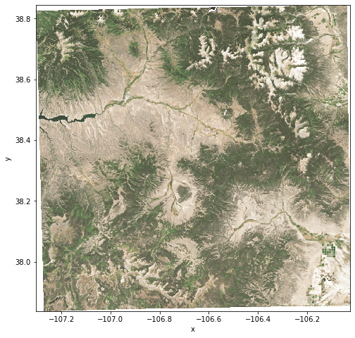
The WGS 84 projection (EPSG: 4326) is commonly used in many geodetic applications, including the Global Positioning System (GPS). WGS 84 displays meridians and parallels as equally spaced vertical and horizontal lines. Converting between x and y coordinates on the map and earth locations is very simple. This projection is very popular for general use. However, the significant distortions inherent to this method make it impractical for many scientific applications.

Follow these steps to use rasterio.warp.reproject to reproject your data to WGS 84 and resample it with the median resampling method.

Step 1: Get shape, CRS, bounds, and transform information from the source dataset and define the destination CRS. Similar to other methods that use rasterio, you can define a resampling method to use when reprojecting the data. To choose median resampling, set med_resampling to rasterio.enums.Resampling.med. This variable will later be used with the resampling parameter.

In [16]:

# source information
src_crs = {"init": scene_data.crs}
src_bounds = scene_data.rio.bounds()
src_transform = scene_data.transform
bands, src_height, src_width = scene_data.shape

# destination CRS
WGS84_crs = {"init": "EPSG:4326"}

# resampling method
med_resampling = rasterio.enums.Resampling.med

Step 2: Calculate the transform and shape of the destination CRS.

In [17]:

WGS84_transform, WGS84_width, WGS84_height = rasterio.warp.calculate_default_transform(
    src_crs, WGS84_crs, src_width, src_height, *src_bounds
)

# array to write results to
WGS84_data = np.zeros((bands, WGS84_height, WGS84_width))

WGS84_transform, WGS84_width, WGS84_height

Out[17]:

(Affine(0.0010196778608226639, 0.0, -107.30489322500127,
        0.0, -0.0010196778608226639, 38.84504275433628),
 1255,
 988)

Step 3: Calculate the coordinates of the destination CRS.

In [18]:

WGS84_coords = _make_coords(
    scene_data, WGS84_transform, WGS84_width, WGS84_height, WGS84_crs
)

WGS84_xs = WGS84_coords["x"]
WGS84_ys = WGS84_coords["y"]

Step 4: Reproject and resample the source data to the destination CRS. Rasterio automatically calculates the target resolution.

In [19]:

rasterio.warp.reproject(
    scene_data,
    WGS84_data,
    src_transform=src_transform,
    src_crs=src_crs,
    dst_transform=WGS84_transform,
    dst_crs=WGS84_crs,
    resampling=med_resampling,
)

Out[19]:

(array([[[0., 0., 0., ..., 0., 0., 0.],
         [0., 0., 0., ..., 0., 0., 0.],
         [0., 0., 0., ..., 0., 0., 0.],
         ...,
         [0., 0., 0., ..., 0., 0., 0.],
         [0., 0., 0., ..., 0., 0., 0.],
         [0., 0., 0., ..., 0., 0., 0.]],
 
        [[0., 0., 0., ..., 0., 0., 0.],
         [0., 0., 0., ..., 0., 0., 0.],
         [0., 0., 0., ..., 0., 0., 0.],
         ...,
         [0., 0., 0., ..., 0., 0., 0.],
         [0., 0., 0., ..., 0., 0., 0.],
         [0., 0., 0., ..., 0., 0., 0.]],
 
        [[0., 0., 0., ..., 0., 0., 0.],
         [0., 0., 0., ..., 0., 0., 0.],
         [0., 0., 0., ..., 0., 0., 0.],
         ...,
         [0., 0., 0., ..., 0., 0., 0.],
         [0., 0., 0., ..., 0., 0., 0.],
         [0., 0., 0., ..., 0., 0., 0.]]]),
 Affine(0.0010196778608226639, 0.0, -107.30489322500127,
        0.0, -0.0010196778608226639, 38.84504275433628))

Step 5: Reconstruct the result as an xarray DataArray.

In [20]:

WGS84_reproj = xr.DataArray(
    WGS84_data,
    dims=["band", "y", "x"],
    coords={"band": scene_data.band, "y": WGS84_ys, "x": WGS84_xs},
)

Step 6: Visualize the projection.

In [21]:

WGS84_img = ms.true_color(*WGS84_reproj, name="epsg=4326")
WGS84_img.plot.imshow(figsize=(8, 8));

Reproject and resample in-memory data with rioxarray's `reproject()`¶

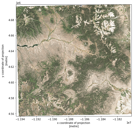
The Web Mercator projection is the de facto standard for Web mapping applications. It is a variant of the Mercator projection and is used by many major online map providers. rioxarray's reproject function is powered by rasterio.warp.reproject(). Let's reproject your data from the CRS of EPSG:6933 to the Web Mercator CRS of EPSG:3857.

Rioxarray's reproject() function accepts resampling and resolution as optional parameters. However, this example uses the library's defaults for resampling: The reproject() function uses the nearest method as its default resampling algorithm. If no resolution is provided, rioxarray calculates the resolution based on the source data and the target CRS.

In [22]:

web_mecator_crs = 3857

web_mecator_reproj = scene_data.rio.reproject(web_mecator_crs)
web_mecator_img = ms.true_color(*web_mecator_reproj, name="epsg=3857")

web_mecator_img.plot.imshow(figsize=(8, 8));

Wrap-up: Compare different reprojections¶

To see how reprojecting and resampling the same source dataset results in very different visualizations, plot all images side by side.

In [23]:

imgs = [cylindrical_img, robinson_img, space_oblique_img, WGS84_img, web_mecator_img]

fig, ax = plt.subplots(nrows=1, ncols=len(imgs), figsize=(20, 15))
for i in range(len(imgs)):
    ax[i].imshow(imgs[i].data)
    ax[i].set_xticks([])
    ax[i].set_yticks([])
    ax[i].set_title(imgs[i].name)

plt.show()

Reprojecting and Resampling¶

Preparation: Create a local Dask cluster¶

Method 1: Reproject and resample while loading with stackstac.stack¶

Method 2: Reproject and resample while loading with rasterio and rioxarray using a WarpedVRT¶

Method 3: Reproject and resample an in-memory array with stackstac.reproject_array¶

Method 4: Reproject and resample an in-memory DataArray with rasterio and rioxarray¶

Reproject and resample in-memory data with rasterio's reproject()¶

Reproject and resample in-memory data with rioxarray's reproject()¶