Radiometric terrain correction qualitative assessment
sarsen radiometric correction implements the gamma flatting algorithm proposed by Small, David (2011). Flattening Gamma: Radiometric Terrain Correction for SAR Imagery. Geoscience and Remote Sensing, IEEE Transactions on. 49. 3081 - 3093. 10.1109/TGRS.2011.2120616
In this notebook, we perform the same qualitative test done by the authors to evaluate the goodness of the gamma flattening correction. For an introduction to terrain correction, see Customizable radiometric terrain corrections of Sentinel-1 products .
Install Dependencies and Imports
Additional dependencies: sarsen==0.9.2
# !pip install sarsen==0.9.2
%matplotlib inline
%config InlineBackend.figure_format = 'retina'


import matplotlib.pyplot as plt
from matplotlib.colors import Normalize
from matplotlib import cm

plt.rcParams["figure.figsize"] = (10, 7)
plt.rcParams["font.size"] = 14
import os
import tempfile

import numpy as np
import xarray as xr
from scipy.stats import gaussian_kde as kde
from sarsen import apps, geocoding, orbit, scene

import adlfs
import planetary_computer
import pystac_client
import stackstac
import rioxarray  # noqa: F401

plt.rcParams["figure.figsize"] = (10, 7)
Processing definitions
# create a temporary directory where to store downloaded data
tmp_dir = tempfile.gettempdir()

# DEM path
dem_path = os.path.join(tmp_dir, "South-of-Redmond-10m.tif")

# path to Sentinel-1 input product in the Planetary Computer
product_folder = "GRD/2021/12/17/IW/DV/S1B_IW_GRDH_1SDV_20211217T141304_20211217T141329_030066_039705_9048"  # noqa: E501

# band to be processed
measurement_group = "IW/VV"

tmp_dir
'/tmp'
Area of interest definition: South-of-Redmond (Seattle, US)
lon, lat = [-121.95, 47.04]
buffer = 0.2
bbox = [lon - buffer, lat - buffer, lon + buffer, lat + buffer]
DEMs discovery
Here we use the DEM with a 10-meter ground sample distance (GDS) available on the Planetary Computer. Note that any DEM supported by GDAL/Proj can be used.
Using pystac_client we can search the Planetary Computer's STAC endpoint for items matching our query parameters.
As multiple DEMs acquired at different times are available in this area, we select the DEMs with 10-meter GDS and perform the average of the remaining DEMs along the time dimension.
catalog = pystac_client.Client.open(
    "https://planetarycomputer.microsoft.com/api/stac/v1",
    modifier=planetary_computer.sign_inplace,
)
search = catalog.search(
    collections="3dep-seamless", bbox=bbox, query={"gsd": {"eq": 10}}
)
items = search.item_collection()
Here we load the data into an xarray DataArray using stackstac.
# select DEMs with resolution 10 meters
dem_raster_all = stackstac.stack(items, bounds=bbox).squeeze()
dem_raster_all
<xarray.DataArray 'stackstac-6fbfb106cd445ae5ea0f677ec80c3c41' (time: 4,
                                                                y: 4321, x: 4321)>
dask.array<getitem, shape=(4, 4321, 4321), dtype=float64, chunksize=(1, 1024, 1024), chunktype=numpy.ndarray>
Coordinates: (12/13)
  * time             (time) datetime64[ns] 2018-02-02 2018-02-08 ... 2020-01-07
    id               (time) <U10 'n48w122-13' 'n47w122-13' ... 'n48w123-13'
    band             <U4 'data'
  * x                (x) float64 -122.2 -122.1 -122.1 ... -121.8 -121.8 -121.8
  * y                (y) float64 47.24 47.24 47.24 47.24 ... 46.84 46.84 46.84
    start_datetime   (time) <U20 '1952-01-01T00:00:00Z' ... '2017-09-14T00:00...
    ...               ...
    proj:shape       object {10812}
    proj:epsg        int64 5498
    threedep:region  <U7 'n40w130'
    gsd              int64 10
    description      <U1849 'This tile of the 3D Elevation Program (3DEP) sea...
    epsg             int64 5498
Attributes:
    spec:        RasterSpec(epsg=5498, bounds=(-122.15000053746, 46.839907613...
    crs:         epsg:5498
    transform:   | 0.00, 0.00,-122.15|\n| 0.00,-0.00, 47.24|\n| 0.00, 0.00, 1...
resolution: 9.2592593e-05DEMs average along the time dimension
dem_raster_geo = dem_raster_all.compute().mean("time")
dem_raster_geo.rio.set_crs(dem_raster_all.rio.crs);
# find the UTM zone and project in UTM
t_srs = dem_raster_geo.rio.estimate_utm_crs()
dem_raster = dem_raster_geo.rio.reproject(t_srs, resolution=(10, 10))
dem_raster
<xarray.DataArray 'stackstac-6fbfb106cd445ae5ea0f677ec80c3c41' (y: 4487, x: 3100)>
array([[1.79769313e+308, 1.79769313e+308, 1.79769313e+308, ...,
        1.79769313e+308, 1.79769313e+308, 1.79769313e+308],
       [1.79769313e+308, 1.79769313e+308, 1.79769313e+308, ...,
        1.79769313e+308, 1.79769313e+308, 1.79769313e+308],
       [1.79769313e+308, 1.79769313e+308, 1.79769313e+308, ...,
        1.79769313e+308, 1.79769313e+308, 1.79769313e+308],
       ...,
       [1.79769313e+308, 1.79769313e+308, 1.79769313e+308, ...,
        1.79769313e+308, 1.79769313e+308, 1.79769313e+308],
       [1.79769313e+308, 1.79769313e+308, 1.79769313e+308, ...,
        1.79769313e+308, 1.79769313e+308, 1.79769313e+308],
       [1.79769313e+308, 1.79769313e+308, 1.79769313e+308, ...,
        1.79769313e+308, 1.79769313e+308, 1.79769313e+308]])
Coordinates:
  * x                (x) float64 5.643e+05 5.643e+05 ... 5.953e+05 5.953e+05
  * y                (y) float64 5.233e+06 5.233e+06 ... 5.188e+06 5.188e+06
    proj:shape       object {10812}
    epsg             int64 5498
    threedep:region  <U7 'n40w130'
    proj:epsg        int64 5498
    gsd              int64 10
    band             <U4 'data'
    description      <U1849 'This tile of the 3D Elevation Program (3DEP) sea...
    spatial_ref      int64 0
Attributes:
_FillValue: 1.7976931348623157e+308# crop DEM to our area of interest and save it
dem_corners = dict(x=slice(579000, 593000), y=slice(5210000, 5195000))
dem_raster = dem_raster.sel(**dem_corners)
dem_raster.rio.to_raster(dem_path)
dem_raster
<xarray.DataArray 'stackstac-6fbfb106cd445ae5ea0f677ec80c3c41' (y: 1500, x: 1400)>
array([[ 840.86486816,  837.69940186,  836.6675415 , ..., 1222.60290527,
        1224.68151855, 1229.60192871],
       [ 847.59912109,  843.43511963,  841.19110107, ..., 1226.77722168,
        1229.88330078, 1235.05480957],
       [ 853.09313965,  849.24804688,  847.56011963, ..., 1231.57214355,
        1235.27197266, 1240.26989746],
       ...,
       [1057.71154785, 1056.44726562, 1053.34716797, ..., 1967.21203613,
        1966.72473145, 1967.17895508],
       [1053.78833008, 1052.40124512, 1049.59545898, ..., 1970.66943359,
        1969.1439209 , 1969.60314941],
       [1049.06298828, 1048.03967285, 1045.55126953, ..., 1973.11730957,
        1971.60437012, 1971.93334961]])
Coordinates:
  * x                (x) float64 5.79e+05 5.79e+05 ... 5.93e+05 5.93e+05
  * y                (y) float64 5.21e+06 5.21e+06 ... 5.195e+06 5.195e+06
    proj:shape       object {10812}
    epsg             int64 5498
    threedep:region  <U7 'n40w130'
    proj:epsg        int64 5498
    gsd              int64 10
    band             <U4 'data'
    description      <U1849 'This tile of the 3D Elevation Program (3DEP) sea...
    spatial_ref      int64 0
Attributes:
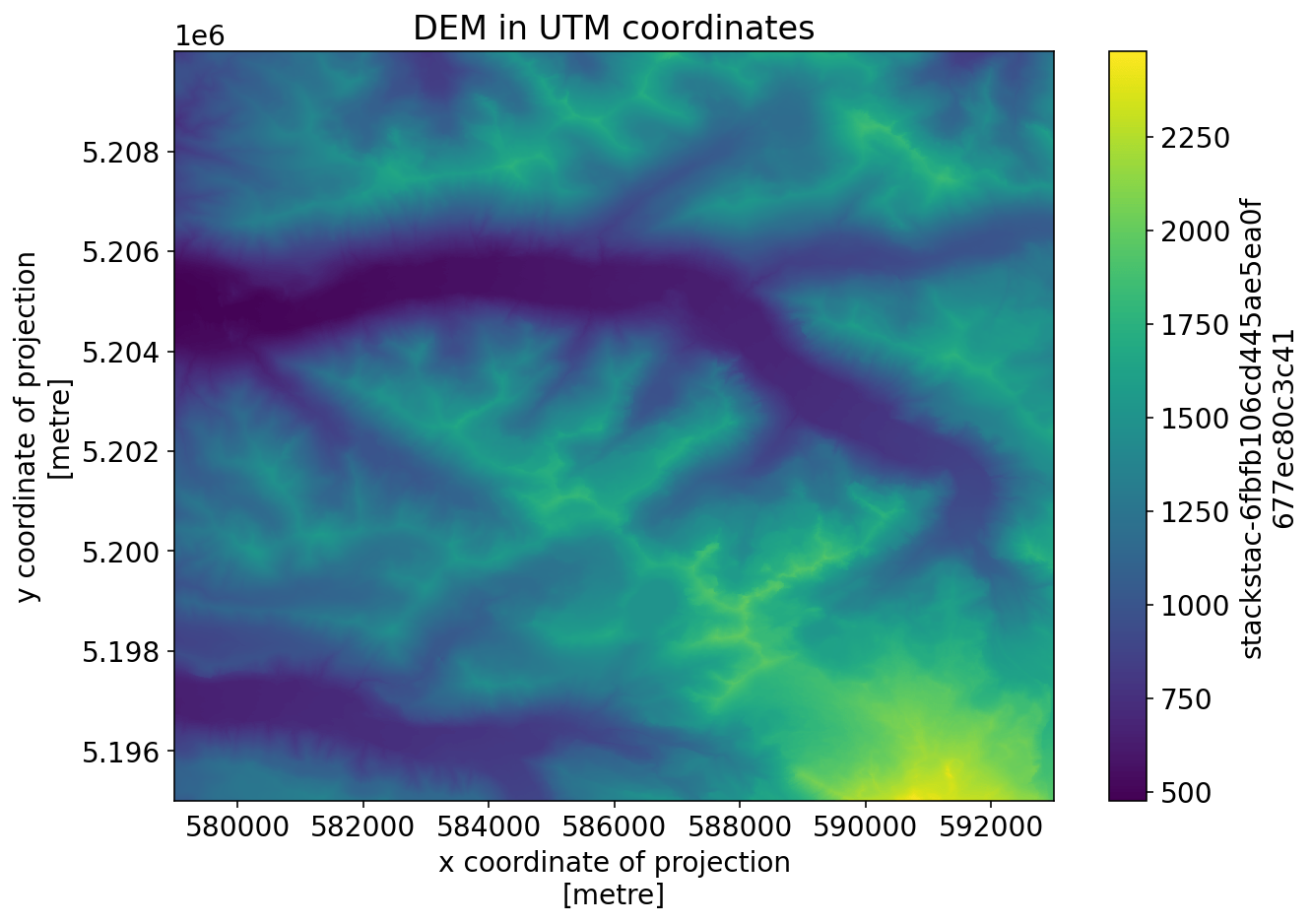
_FillValue: 1.7976931348623157e+308dem_raster.plot()
_ = plt.title("DEM in UTM coordinates")
Define GRD parameters
grd_account_name = "sentinel1euwest"
grd_storage_container = "s1-grd"
grd_product_folder = f"{grd_storage_container}/{product_folder}"
grd_local_path = os.path.join(tmp_dir, product_folder)
Retrieve Sentinel-1 GRD
grd_token = planetary_computer.sas.get_token(
    grd_account_name, grd_storage_container
).token
grd_fs = adlfs.AzureBlobFileSystem(grd_account_name, credential=grd_token)
grd_fs.ls(f"{grd_product_folder}/manifest.safe")
['s1-grd/GRD/2021/12/17/IW/DV/S1B_IW_GRDH_1SDV_20211217T141304_20211217T141329_030066_039705_9048/manifest.safe']
grd_fs.get(grd_product_folder, grd_local_path, recursive=True)
!ls -d {grd_local_path}
/tmp/GRD/2021/12/17/IW/DV/S1B_IW_GRDH_1SDV_20211217T141304_20211217T141329_030066_039705_9048
Process
GTC
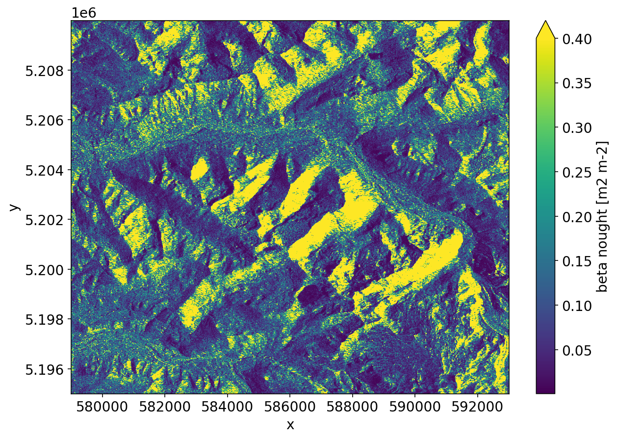
Here we compute the geometric terrain correction.
Input parameters:
product_urlpath: product pathmeasurement_group: band to be processed in the form {swath}/{polarization} (see xarray-sentinel for more details)dem_urlpath: path to the input DEM. sarsen supports all DEMs supported by GDAL/Proj for ECEF-translation.interp_method: interpolation method, sarsen supports all interpolation methods supported by xarray.Dataset.interpchunks: dask chunksoutput_urlpath: output path
The output is the input SAR image resampled on DEM coordinates
gtc_path = os.path.basename(product_folder) + ".GTC.tif"

gtc = apps.terrain_correction(
    grd_local_path,
    measurement_group,
    dem_path,
    interp_method="nearest",
    override_product_files="{dirname}/{prefix}{swath}-{polarization}{ext}",
    chunks=2048,
    output_urlpath=gtc_path,
)
_ = gtc.plot(vmax=0.4)
RTC
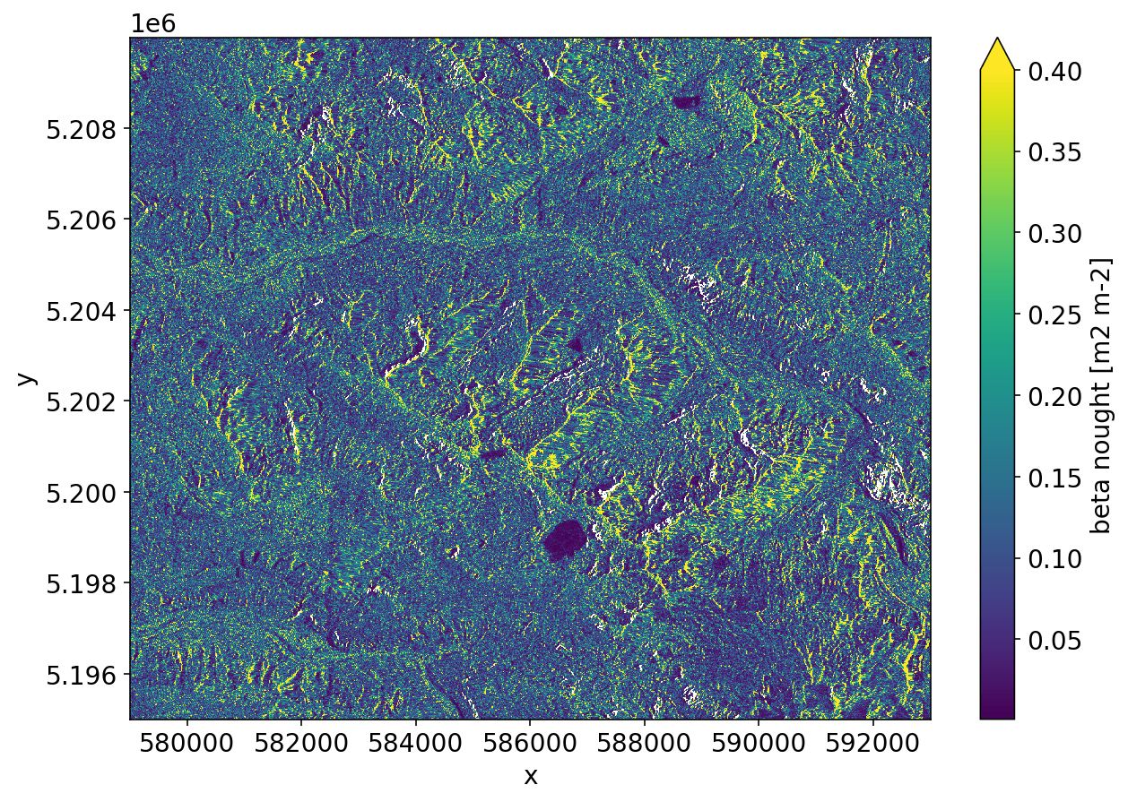
sarsen implements the radiometric terrain-correction Gamma Flattening algorithm.
Input parameters
correct_radiometry:correct_radiometry: defaultNone. Ifcorrect_radiometry=Nonethe radiometric terrain correction is not applied.correct_radiometry=gamma_bilinearapplies the gamma flattening classic algorithm using bilinear interpolation to compute the weights.correct_radiometry=gamma_nearestapplies the gamma flattening using nearest neighbours instead of bilinear interpolation. 'gamma_nearest' significantly reduces the processing time.grouping_area_factor: scaling factor for the size of the image pixel where the areas are summed. By default, thegrouping_area_factoris(1, 1), which corresponds to Sentinel-1 input product pixel size. Thegrouping_area_factorshall be increased if the DEM resolution is lower than the Sentinel-1 input product resolution to avoid gaps and distortions the normalization factor. It can be also used to to speed up the computation or the DEM resolution is lower than the Sentinel-1 input product resolution.
Note: The grouping_area_factor can be increased (i) to speed up the processing or (ii) when the input DEM resolution is low. The Gamma Flattening usually works properly if the pixel size of the input DEM is much smaller than the pixel size of the input Sentinel-1 product. Otherwise, the output may have radiometric distortions. This problem can be avoided by increasing the grouping_area_factor. Be aware that grouping_area_factor too high may degrade the final result.
import warnings

warnings.filterwarnings("ignore", "divide by zero", RuntimeWarning)
rtc_path = os.path.basename(grd_local_path) + ".RTC.tif"

rtc = apps.terrain_correction(
    grd_local_path,
    measurement_group,
    dem_path,
    interp_method="nearest",
    override_product_files="{dirname}/{prefix}{swath}-{polarization}{ext}",
    correct_radiometry="gamma_nearest",
    output_urlpath=rtc_path,
    grouping_area_factor=(1, 1),
)
_ = rtc.plot(vmax=0.4)
Gamma vs Local incidence Angle
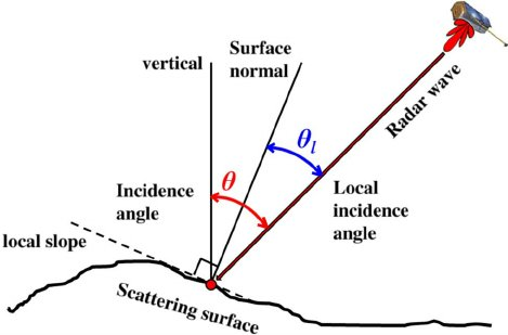
The backscattering depends on the ground material, the roughness and the local incidence angle. Small values of the local incidence angle correspond usually to higher values of backscattering, while high values of radar incidence angle corresponds to zones with low backscattering. The aim of the radiometric terrain correction is to remove the contribution due to the local incidence angle. For evaluating the goodness of the radiometric correction we will compare the incidence angle versus backscattering before and after the correction.
Compute local incidence angle and ellipsoid incidence angle
dem = scene.open_dem_raster(dem_path)


orbit_ecef = xr.open_dataset(
    grd_local_path,
    engine="sentinel-1",
    group=f"{measurement_group}/orbit",
    override_product_files="{dirname}/{prefix}{swath}-{polarization}{ext}",
)
dem_ecef = scene.convert_to_dem_ecef(dem, source_crs=t_srs)
dem_ecef_1 = scene.convert_to_dem_ecef(dem + 1, source_crs=t_srs)
ellissoid_normal = dem_ecef - dem_ecef_1
acquisition = apps.simulate_acquisition(
    dem_ecef, orbit_ecef.position, coordinate_conversion=None, correct_radiometry=True
)
oriented_area = scene.compute_dem_oriented_area(dem_ecef)
dem_normal = -oriented_area / np.sqrt(xr.dot(oriented_area, oriented_area, dims="axis"))

# compute direction target sensor
orbit_interpolator = orbit.OrbitPolyfitIterpolator.from_position(orbit_ecef.position)
position_ecef = orbit_interpolator.position()
velocity_ecef = orbit_interpolator.velocity()
acquisition = geocoding.backward_geocode(dem_ecef, orbit_ecef.position, velocity_ecef)
slant_range = np.sqrt((acquisition.dem_distance**2).sum(dim="axis"))
dem_direction = acquisition.dem_distance / slant_range
angle = np.arccos(xr.dot(dem_normal, dem_direction, dims="axis"))
ellipsoid_incidence = np.arccos(xr.dot(ellissoid_normal, dem_direction, dims="axis"))
Load Data
ellipsoid_incidence = ellipsoid_incidence.load()
angle = angle.load()
gtc = gtc.load()
rtc = rtc.load()
GTC and RTC distribution of foreslope, backslope, and flat terrain
We classify taking into account the local incidence angle and the ellipsoid incidence angle the image in three zone:
- foreslope, small incidence angles that correspond to high backscattering zones.
- flat terrain
- backslope, big incidence angles that correspond to low backscattering zones
We will show that the radiometric correction mitigate the effect of the foreslope and backslope.
# foreslope backslope and flat terrain
gtc_foreslope = xr.where(angle < ellipsoid_incidence - 0.20, gtc, np.nan)
gtc_backslope = xr.where(angle > ellipsoid_incidence + 0.20, gtc, np.nan)
gtc_flat = xr.where(
    (angle < ellipsoid_incidence + 0.20) & (angle > ellipsoid_incidence - 0.20),
    gtc,
    np.nan,
)

rtc_foreslope = xr.where(angle < ellipsoid_incidence - 0.20, rtc, np.nan)
rtc_backslope = xr.where(angle > ellipsoid_incidence + 0.20, rtc, np.nan)
rtc_flat = xr.where(
    (angle < ellipsoid_incidence + 0.20) & (angle > ellipsoid_incidence - 0.20),
    rtc,
    np.nan,
)
f, axes = plt.subplots(nrows=1, ncols=3, figsize=(30, 9))

dem_raster.plot(ax=axes[0])
axes[0].grid(c="red")
axes[0].set_title("DEM")

gtc.plot(ax=axes[1], vmax=0.4)
axes[1].grid(c="red")
axes[1].set_title("GTC")


angle.plot(ax=axes[2])
axes[2].grid(c="red")
axes[2].set_title("Incidence Angle")

plt.tight_layout()

f, axes = plt.subplots(nrows=1, ncols=3, figsize=(30, 9))

gtc_backslope.plot(ax=axes[0], vmax=0.4)
axes[0].grid(c="red")
axes[0].set_title("GTC basckslope")

gtc_foreslope.plot(ax=axes[1], vmax=0.4)
axes[1].grid(c="red")
axes[1].set_title("GTC foreslope")


gtc_flat.plot(ax=axes[2], vmax=0.4)
axes[2].grid(c="red")
axes[2].set_title("GTC flat terrain")


plt.tight_layout()

GTC and RTC distribution of foreslope backslope and flat terrain in db
gtc_backslope_db = np.log(gtc_backslope)
gtc_foreslope_db = np.log(gtc_foreslope)
gtc_flat_db = np.log(gtc_flat)

rtc_backslope_db = np.log(rtc_backslope)
rtc_foreslope_db = np.log(rtc_foreslope)
rtc_flat_db = np.log(rtc_flat)
f, axes = plt.subplots(nrows=1, ncols=2, figsize=(30, 12))

gtc_backslope_db_h = xr.plot.hist(
    gtc_backslope_db,
    range=[-10, 5],
    bins=50,
    color=[0, 1, 0, 0.4],
    density=True,
    ax=axes[0],
    label="backslope",
)
gtc_foreslope_db_h = xr.plot.hist(
    gtc_foreslope_db,
    range=[-10, 5],
    bins=50,
    color=[1, 0, 0, 0.4],
    density=True,
    ax=axes[0],
    label="foreslope",
)
gtc_flat_db_h = xr.plot.hist(
    gtc_flat_db,
    range=[-10, 5],
    bins=50,
    color=[0, 0, 1, 0.4],
    density=True,
    ax=axes[0],
    label="flat",
)

rtc_backslope_db_h = xr.plot.hist(
    rtc_backslope_db,
    range=[-10, 5],
    bins=50,
    color=[0, 1, 0, 0.4],
    density=True,
    ax=axes[1],
    label="backslope",
)
rtc_foreslope_db_h = xr.plot.hist(
    rtc_foreslope_db,
    range=[-10, 5],
    bins=50,
    color=[1, 0, 0, 0.4],
    density=True,
    ax=axes[1],
    label="foreslope",
)
rtc_flat_db_h = xr.plot.hist(
    rtc_flat_db,
    range=[-10, 5],
    bins=50,
    color=[0, 0, 1, 0.4],
    density=True,
    ax=axes[1],
    label="flat",
)
axes[0].legend()
axes[1].legend()

axes[0].set_title("GTC distribution")
axes[0].set_xlabel("beta DB")

axes[1].set_title("RTC distribution")
axes[1].set_xlabel("gamma_T DB")
Text(0.5, 0, 'gamma_T DB')
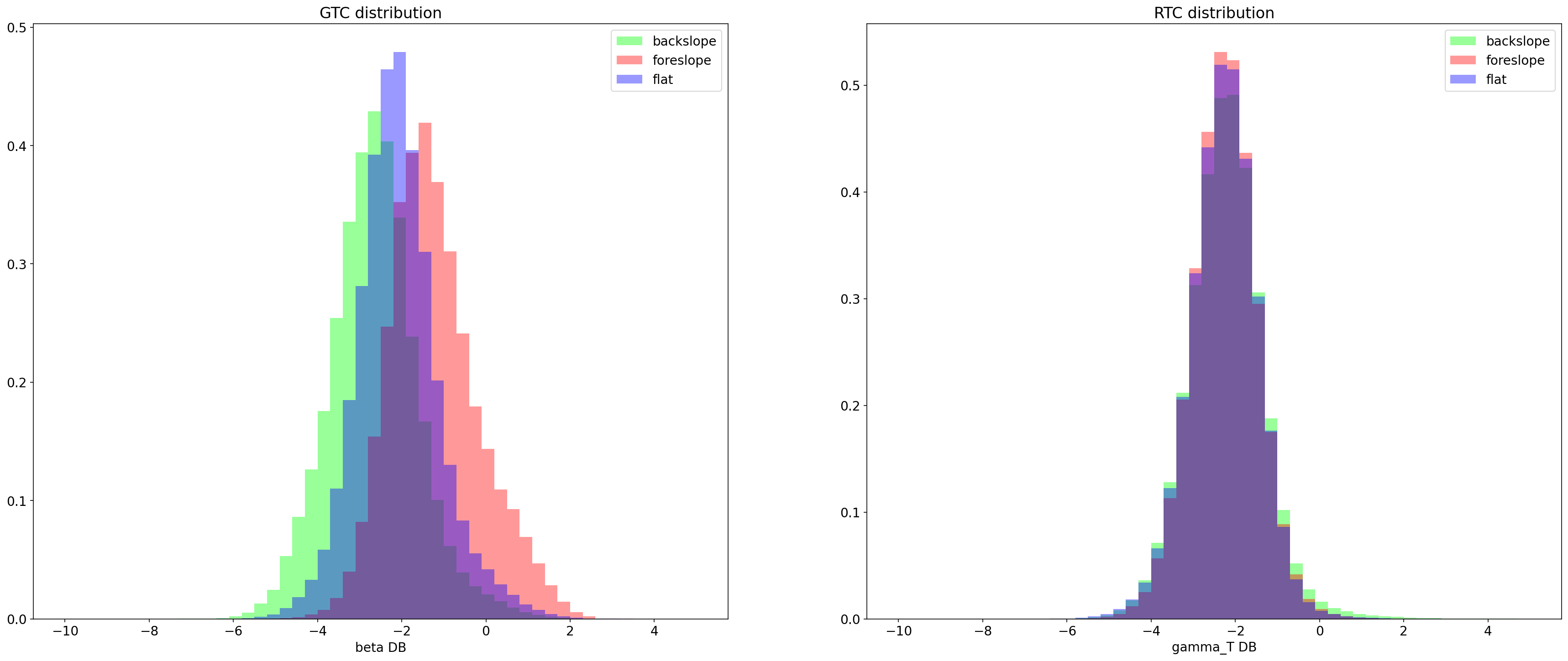
Before the radiometic correction the distribution of backslope flat terrain and foreslope are separate, after they overlap completely.
RTC and GTC scatterplots incidence angle vs backcattering
We compare the incidence_angle-backscattering scatterplots of the GTC and the RTC to show that in the former there is a correlation between the incidence angle and backscattering, while in the RTC the correlation has been removed.
def makeColours(vals):
    colours = np.zeros((len(vals), 3))
    norm = Normalize(vmin=vals.min(), vmax=vals.max())

    # Can put any colormap you like here.
    colours = [cm.ScalarMappable(norm=norm, cmap="plasma").to_rgba(val) for val in vals]

    return colours


def plot_density(x, y, ax=None):
    if ax is None:
        ax = plt
    mask = np.logical_and(np.isfinite(y), np.isfinite(x))
    samples = np.stack([x[mask], y[mask]])

    densObj = kde(samples)
    colours = makeColours(densObj.evaluate(samples))
    fig = ax.scatter(samples[0], samples[1], color=colours)
    return fig
gtc_db = np.log(gtc).load()
rtc_db = np.log(rtc).load()
angle = angle.load()
f, axes = plt.subplots(nrows=1, ncols=2, figsize=(30, 12))

fig = plot_density(
    angle[::10, ::10].data.ravel(), gtc_db[::10, ::10].data.ravel(), ax=axes[0]
)
fig = plot_density(
    angle[::10, ::10].data.ravel(), rtc_db[::10, ::10].data.ravel(), ax=axes[1]
)

axes[0].set_title("GTC")
axes[0].set_ylabel("beta DB")
axes[0].set_xlabel("local incidence angle")

axes[1].set_title("RTC")
axes[1].set_ylabel("gamma_T DB")
axes[1].set_xlabel("local incidence angle")
Text(0.5, 0, 'local incidence angle')
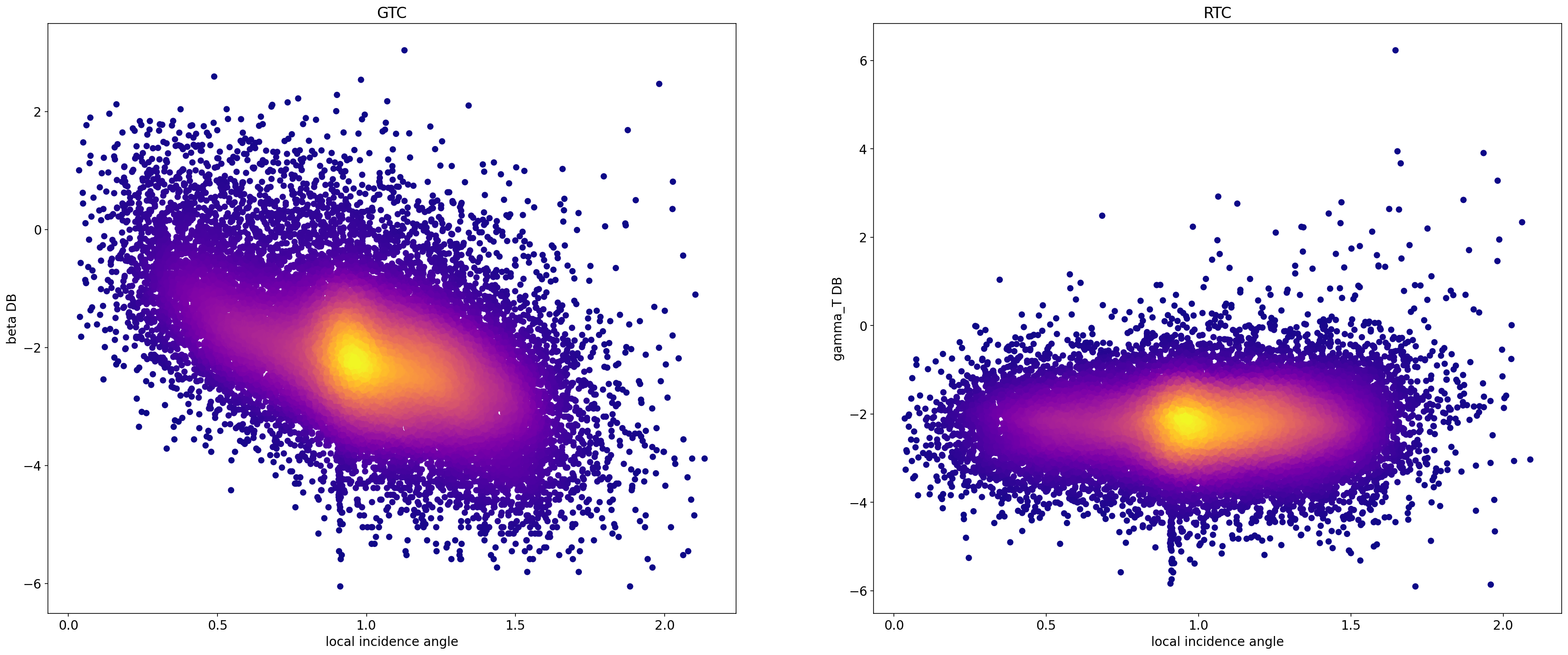
Note that in the first plot there is a clear correlation between the angle of incidence and backscattering, while in the second graph there is no correlation.