Geospatial Classification¶

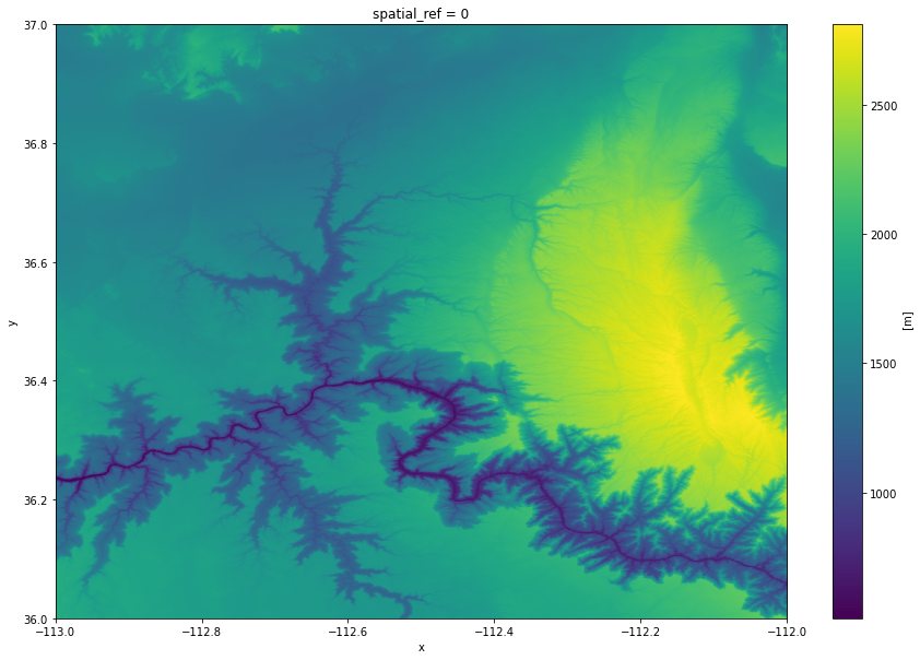
In this tutorial, you'll learn how to use different classification methods with xarray-spatial to classify the terrain elevation levels of the Grand Canyon, using data from the NASADEM dataset.

Geospatial data classification algorithms assign groups of data to categories, or classes, for further processing. Classification is used when grouping data points into classes for different colored areas on a choropleth map, for example. xarray-spatial is a raster analysis tool and contains different classification methods.

This tutorial walks you through:

1. Loading and rendering the area of interest data using the Grand Canyon's latitude and longitude.
2. Classifying the data using xarray-spatial's natural breaks, equal interval, quantile, and reclassify functions.

This tutorial uses the NASADEM dataset, which provides global topographic data at 1 arc-second (~30m) horizontal resolution. The data is derived primarily from data captured via the Shuttle Radar Topography Mission (SRTM) and is stored on Azure Storage in cloud-optimized GeoTIFF format. The area of interest roughly covers the Grand Canyon National Park.

Load the area of interest data¶

We'll use pystac-client to search for the COG covering Grand Canyon National Park.

This item's data can be read in using xarray's open_rasterio function to load the data into an array:

Classify elevation data¶

Classify with natural_breaks()¶

Now let's use the natural breaks function to classify data with the Jenks natural breaks classification method. This method is designed to distribute data into classes according to clusters that form a "natural" group within the data. The algorithm minimizes the average deviation from the class mean while also maximizing the deviation from the means of the other groups. Therefore, it is generally not recommended for data with low variance.

The num_sample parameter allows you to control how many values to sample while calculating the groupings and has a big impact on performance. Fine-tuning num_sample requires an understanding of confidence intervals / margin of error along with general knowledge of the distribution of the data (e.g. are values normally distributed?). For this example we've set num_samples=20000.

You can see in the image above that the different elevation levels of the Grand Canyon are now identified by a limited number of distinct colors. Each color represents a range of values within the classified data. For example, the dark blue color areas represent the smallest elevation levels with around 700m of altitude, the yellow color areas represent elevation levels of around 1700m, and the white color areas represent the highest elevations of around 2500m of altitude.

Classify with equal_interval()¶

To classify data into sets based on intervals of equal width, use the equal interval function. The equal interval classification is useful in cases where you want to highlight the relative prevalence of values. As each grouping has the same range, the number of values in each group will differ.

Classify with quantile()¶

To classify data based on quantile groups of equal size, use the quantile function. With quantile classification, each class contains the same number of data points. This means that each class is equally represented on the map. However, intervals of uneven sizes can lead to an over-weighting of outliers and other effects.

Use custom bins with reclassify¶

To define your own arbitrary bins to classify data, use the reclassify function. This function is helpful to highlight specific sections of your data, for example. Use reclassify() to only visualize elevations greater than 2500m:

Next steps: classify different datasets¶

The Planetary Computer Data Catalog includes petabytes of environmental monitoring data. All data sets are available in consistent, analysis-ready formats. You can access them through APIs as well as directly via Azure Storage.

Try using xarray-spatial's classification methods with these datasets:

Daymet Gridded temperature data across North America Get Daymet temperature data

GBIF Species occurrences shared through the Global Biodiversity Information Facility Get GBIF occurrence data