Zonal Statistics¶

In this tutorial, you'll learn how to use xarray-spatial to work with zonal statistics. Zonal statistics help you better understand data from one source by analyzing it for different zones defined by another source. This operation uses two datasets: One dataset, the zones raster, defines one or more zones. A second dataset, the values raster, contains the data you want to analyze for each of the zones defined by the first dataset. If you're familiar with SQL or dataframe libraries like pandas, this is similar to a group by operation: you essentially group the values raster by the zones raster.

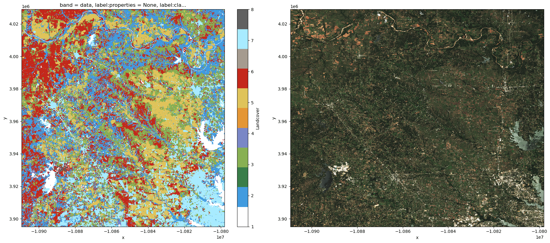
In this tutorial, we'll use the Esri / Observatory 10-Meter Land Cover dataset, which classifies pixels into one of ten classes, as the zones raster. Our values raster will be Normalized difference vegetation index (NDVI), derived from Sentinel-2 Level 2-A.

In [1]:

import numpy as np

import planetary_computer
import pystac_client
import stackstac
import rasterio.features

import matplotlib.pyplot as plt
from matplotlib.colors import ListedColormap

from xrspatial.multispectral import true_color

from xrspatial.classify import equal_interval
from xrspatial.zonal import stats as zonal_stats
from xrspatial.zonal import crosstab as zonal_crosstab

Preparation: Create a local Dask cluster¶

We'll make a local Dask cluster to process the data in parallel.

In [2]:

from dask.distributed import Client

client = Client()
print(f"/proxy/{client.scheduler_info()['services']['dashboard']}/status")

/proxy/8787/status

To follow the progress of your computation, you can access the Dask Dashboard at the URL from the previous cell's output.

Load and coregister data¶

The area of interest covers Lake Bridgeport, Texas, USA. We'll use pystac-client to find items covering that area, and stackstac to load the items into a DataArray.

In [3]:

catalog = pystac_client.Client.open(
    "https://planetarycomputer.microsoft.com/api/stac/v1/",
    modifier=planetary_computer.sign_inplace,
)

bounds = (-98.00080760573508, 32.99921674609716, -96.9991860639418, 34.000729644613706)

landcover_search = catalog.search(collections=["io-lulc"], bbox=bounds)
landcover_items = landcover_search.item_collection()

landcover_data = (
    stackstac.stack(
        landcover_items,
        epsg=3857,
        bounds_latlon=bounds,
        dtype="int8",
        fill_value=0,
        chunksize=2048,
        resolution=100,
    )
    .pipe(stackstac.mosaic, nodata=0)
    .squeeze()
    .rename("Landcover")
    .persist()
)
landcover_data

Out[3]:

<xarray.DataArray 'Landcover' (y: 1338, x: 1115)>
dask.array<getitem, shape=(1338, 1115), dtype=int8, chunksize=(1338, 1115), chunktype=numpy.ndarray>
Coordinates:
    band               <U4 'data'
  * x                  (x) float64 -1.091e+07 -1.091e+07 ... -1.08e+07 -1.08e+07
  * y                  (y) float64 4.029e+06 4.029e+06 ... 3.895e+06 3.895e+06
    label:properties   object None
    label:classes      object {'name': '', 'classes': ['nodata', 'water', 'tr...
    label:description  <U4 'lulc'
    proj:shape         object {74688, 101302}
    label:type         <U6 'raster'
    start_datetime     <U20 '2020-01-01T00:00:00Z'
    end_datetime       <U20 '2021-01-01T00:00:00Z'
    raster:bands       object {'nodata': 0, 'spatial_resolution': 10}
    epsg               int64 3857
Attributes:
    spec:        RasterSpec(epsg=3857, bounds=(-10909400, 3895100, -10797900,...
    crs:         epsg:3857
    transform:   | 100.00, 0.00,-10909400.00|\n| 0.00,-100.00, 4028900.00|\n|...
    resolution:  100

The landcover data includes some class labels, which we'll use to label the outputs later on.

In [4]:

landcover_labels = dict(
    enumerate(landcover_data.coords["label:classes"].item()["classes"])
)
landcover_labels

Out[4]:

{0: 'nodata',
 1: 'water',
 2: 'trees',
 3: 'grass',
 4: 'flooded veg',
 5: 'crops',
 6: 'scrub',
 7: 'built area',
 8: 'bare',
 9: 'snow/ice',
 10: 'clouds'}

Finally, the landcover COGs also include a colormap.

In [5]:

class_count = len(landcover_labels)

with rasterio.open(landcover_items[0].assets["data"].href) as src:
    landcover_colormap_def = src.colormap(1)  # get metadata colormap for band 1
    landcover_colormap = [
        np.array(landcover_colormap_def[i]) / 255 for i in range(class_count)
    ]

landcover_cmap = ListedColormap(landcover_colormap)

Sentinel data¶

Now we'll do the same thing, only for sentinel-2-l2a items from July 2020. We'll also try to select some not-too cloudy items and mosaic over time to remove as many clouds as possible.

In [6]:

sentinel_search = catalog.search(
    collections=["sentinel-2-l2a"],
    bbox=bounds,
    datetime="2020-07-01/2020-07-30",
    query={
        "eo:cloud_cover": {
            "lt": 10,
        }
    },
)

sentinel_items = sentinel_search.item_collection()

We'll need the zones and values rasters to be in the same CRS and resolution, so we'll make sure to pass those values while we're loading the data with stackstac (see Coregistration for more).

In [7]:

sentinel_data = (
    (
        stackstac.stack(
            sentinel_items,
            resolution=landcover_data.resolution,
            epsg=landcover_data.spec.epsg,
            bounds=landcover_data.spec.bounds,
            assets=["B02", "B03", "B04", "B08"],  # blue, green, red, nir
            chunksize=2048,
        )
        .assign_coords(band=lambda x: x.common_name.rename("band"))  # use common names
        .where(lambda x: x > 0, other=np.nan)  # Sentinels uses 0 as nodata
    )
    .median(dim="time", keep_attrs=True)
    .persist()
)
sentinel_data

Out[7]:

<xarray.DataArray 'stackstac-0446337b875acfbadb5267ecf6c67e26' (band: 4,
                                                                y: 1338, x: 1115)>
dask.array<nanmedian, shape=(4, 1338, 1115), dtype=float64, chunksize=(1, 669, 1115), chunktype=numpy.ndarray>
Coordinates: (12/19)
  * band                                     (band) <U5 'blue' 'green' ... 'nir'
  * x                                        (x) float64 -1.091e+07 ... -1.08...
  * y                                        (y) float64 4.029e+06 ... 3.895e+06
    s2:datatake_type                         <U8 'INS-NOBS'
    constellation                            <U10 'Sentinel 2'
    sat:orbit_state                          <U10 'descending'
    ...                                       ...
    proj:shape                               object {10980}
    title                                    (band) <U20 'Band 2 - Blue - 10m...
    common_name                              (band) <U5 'blue' 'green' ... 'nir'
    center_wavelength                        (band) float64 0.49 0.56 ... 0.842
    full_width_half_max                      (band) float64 0.098 ... 0.145
    epsg                                     int64 3857
Attributes:
    spec:        RasterSpec(epsg=3857, bounds=(-10909400, 3895100, -10797900,...
    crs:         epsg:3857
    transform:   | 100.00, 0.00,-10909400.00|\n| 0.00,-100.00, 4028900.00|\n|...
    resolution:  100

Create a true color image for the Sentinel data:

In [8]:

sentinel_img = true_color(
    sentinel_data.sel(band="red"),
    sentinel_data.sel(band="green"),
    sentinel_data.sel(band="blue"),
    c=30,
    th=0.075,
    name="True color (Sentinel)",
)

In [9]:

fig, (ax1, ax2) = plt.subplots(ncols=2, figsize=(18, 8))

landcover_data.plot.imshow(ax=ax1, cmap=landcover_cmap)
sentinel_img.plot.imshow(ax=ax2)
plt.tight_layout()

As a final bit of setup, we'll compute NDVI for the sentinel-2 scene. This will be our values raster when we compute zonal statistics later on.

In [10]:

red, nir = sentinel_data.sel(band=["red", "nir"])
ndvi = ((nir - red) / (nir + red)).persist()
ndvi

Out[10]:

<xarray.DataArray 'stackstac-0446337b875acfbadb5267ecf6c67e26' (y: 1338, x: 1115)>
dask.array<truediv, shape=(1338, 1115), dtype=float64, chunksize=(669, 1115), chunktype=numpy.ndarray>
Coordinates: (12/14)
  * x                                        (x) float64 -1.091e+07 ... -1.08...
  * y                                        (y) float64 4.029e+06 ... 3.895e+06
    s2:datatake_type                         <U8 'INS-NOBS'
    constellation                            <U10 'Sentinel 2'
    sat:orbit_state                          <U10 'descending'
    s2:saturated_defective_pixel_percentage  float64 0.0
    ...                                       ...
    s2:processing_baseline                   <U5 '02.12'
    s2:degraded_msi_data_percentage          float64 0.0
    s2:product_type                          <U7 'S2MSI2A'
    gsd                                      float64 10.0
    proj:shape                               object {10980}
    epsg                                     int64 3857

Compute zonal statistics¶

Now that we have our zones raster (the landcover DataArray) and our values raster (NDVI derived from the Sentinel composite), we're ready to compute zonal stats.

We'll use xrspatial.zonal.stats to find a few summary statistics for each landcover class.

In [11]:

quantile_stats = (
    zonal_stats(
        zones=landcover_data,
        values=ndvi,
        stats_funcs=["mean", "max", "min", "count"],
    )
    .compute()
    .set_index("zone")
    .rename(landcover_labels)
)
quantile_stats.style.background_gradient()

/srv/conda/envs/notebook/lib/python3.10/site-packages/dask/dataframe/multi.py:1260: UserWarning: Concatenating dataframes with unknown divisions.
We're assuming that the indices of each dataframes are 
 aligned. This assumption is not generally safe.
  warnings.warn(

Out[11]:

	mean	max	min	count
zone
water	0.017884	0.846885	-0.443129	45139.000000
trees	0.743280	0.900511	-0.277344	339387.000000
grass	0.583749	0.877947	-0.140070	323999.000000
flooded veg	0.547517	0.860692	-0.334288	1573.000000
crops	0.510050	0.882642	-0.252886	241772.000000
scrub	0.577787	0.879797	-0.375246	336952.000000
built area	0.494027	0.878849	-0.388387	198272.000000
bare	0.087579	0.704829	-0.375067	4776.000000

Unsurprisingly, landcover classes like "trees" and "grass" have relatively high NDVI values. Classes like "water" and "bare" are relatively low.

Compute zonal cross-tabulation statistics¶

xrspatial.zonal.crosstab calculates cross-tabulated areas between the zone raster and value raster. This function requires a 2D zone raster and a categorical value raster of 2D or 3D data.

The crosstab function calculates different cross-tabulation statistics. It has an agg parameter to define which aggregation method to use. It returns a DataFrame where each row represents a zone from the zone raster and each column represents a category from the value raster.

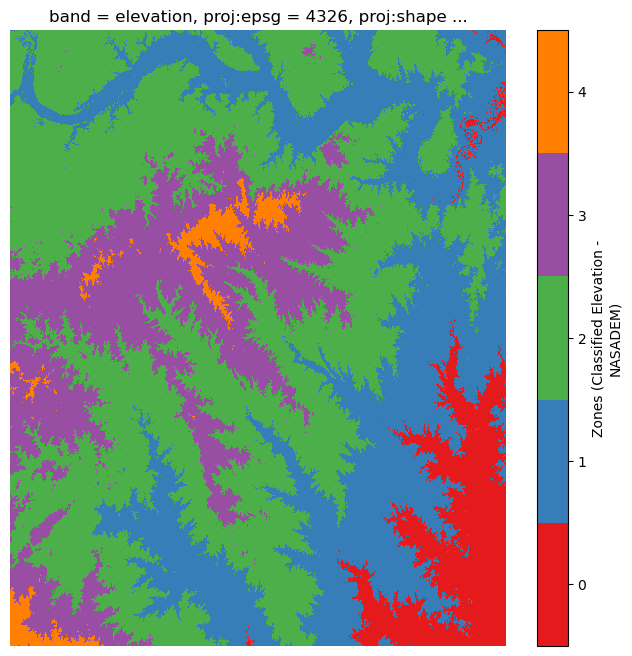
This example uses the NASADEM elevation zones as its zone raster and the Esri Land Cover data as its categorical value raster. The resulting DataFrame will show the percentage of each land cover category for each of the five elevation zones.

In [12]:

nasadem_search = catalog.search(collections=["nasadem"], bbox=bounds)
nasadem_items = nasadem_search.item_collection()

nasadem_data = (
    stackstac.stack(
        nasadem_items,
        epsg=landcover_data.spec.epsg,
        resolution=landcover_data.resolution,
        bounds=landcover_data.spec.bounds,
        chunksize=2048,
    )
    .pipe(stackstac.mosaic)
    .squeeze()
    .persist()
).rename("Elevation (NASADEM)")
nasadem_data

Out[12]:

<xarray.DataArray 'Elevation (NASADEM)' (y: 1338, x: 1115)>
dask.array<getitem, shape=(1338, 1115), dtype=float64, chunksize=(1338, 1115), chunktype=numpy.ndarray>
Coordinates:
    band        <U9 'elevation'
  * x           (x) float64 -1.091e+07 -1.091e+07 ... -1.08e+07 -1.08e+07
  * y           (y) float64 4.029e+06 4.029e+06 ... 3.895e+06 3.895e+06
    proj:epsg   int64 4326
    proj:shape  object {3601}
    title       <U9 'Elevation'
    epsg        int64 3857
Attributes:
    spec:        RasterSpec(epsg=3857, bounds=(-10909400, 3895100, -10797900,...
    crs:         epsg:3857
    transform:   | 100.00, 0.00,-10909400.00|\n| 0.00,-100.00, 4028900.00|\n|...
    resolution:  100

Now let's discretize it into five zones.

In [13]:

num_zones = 5
elevation_cmap = ListedColormap(plt.get_cmap("Set1").colors[:num_zones])

quantile_zones = equal_interval(
    nasadem_data, k=num_zones, name="Zones (Classified Elevation - NASADEM)"
)
fig, ax = plt.subplots(figsize=(8, 8))
img = quantile_zones.plot.imshow(cmap=elevation_cmap, ax=ax)
img.colorbar.set_ticks([0.4, 1.2, 2.0, 2.8, 3.6])
img.colorbar.set_ticklabels(range(5))

ax.set_axis_off()

Finally, calculate the cross-tabulation statistics and display a table demonstrating how the land cover categories are distributed over each of the five elevation zones. Set values for zone_ids and cat_ids to indicate the zones and the categories of interest. In this example, we'll use all the available zones and categories.

In [14]:

crosstab = (
    zonal_crosstab(
        zones=quantile_zones,
        values=landcover_data,
        agg="percentage",
    )
    .rename(columns=landcover_labels)
    .compute()
    .set_index("zone")
)

crosstab.style.background_gradient()

Out[14]:

	water	trees	grass	flooded veg	crops	scrub	built area	bare
zone
0.000000	19.270796	16.616853	10.577962	0.395211	7.421678	7.088585	38.439863	0.189053
1.000000	2.027249	23.448931	22.147768	0.109607	20.129374	13.828654	17.774741	0.533675
2.000000	2.075033	20.599665	23.654604	0.090979	16.611000	27.911911	8.759015	0.297792
3.000000	0.596741	27.804037	21.278863	0.029319	14.013572	28.321761	7.864891	0.090816
4.000000	0.216216	34.702703	19.106518	0.003180	6.206677	32.282989	7.033386	0.448331

Next steps: analyze different datasets¶

The Planetary Computer Data Catalog includes petabytes of environmental monitoring data. All data sets are available in consistent, analysis-ready formats. You can access them through APIs as well as directly via Azure Storage.

Try using xrspatial.zonal.stats and xrspatial.zonal.crosstab with different datasets from the Data Catalog. For example, try using the land cover categories from the Esri 10m Land Cover dataset as zonal raster. Or try using the Map of Biodiversity Importance (MoBI) dataset as a values raster.

There are also other zonal functions in xarray spatial to use with your datasets.