Introduction to Thermodynamics and Statistical Physics
In this lecture, we are going to discuss:
- Applications of the energy equipartition theorem.
- The partition function.
Applications of Equipartition of Energy
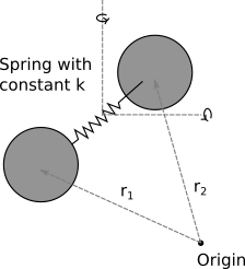
Vibrational energy in a diatomic gas: Now imagine that same gas, but where the bond is no longer rigid, but instead acts like a spring with spring constant k. This adds gives another 2 terms:
$$
\frac{1}{2}\mu ({\bf \dot{r_1}-\dot{r_2}})^2 + \frac{1}{2} k (|{\bf \dot{r_1}-\dot{r_2}}|-l_0)^2
$$
where k is an imagined spring constant, $l_0$ is the equilibrium molecular bond length, and $\mu$ is the reduced mass of the system. This means the total energy is
$$
E = \frac{1}{2} mv_x^2+\frac{1}{2} mv_y^2+\frac{1}{2} mv_z^2+\frac{L_1^2}{2I_1} + \frac{L_2^2}{2I_2}+\frac{1}{2}\mu ({\bf \dot{r_1}-\dot{r_2}})^2 + \frac{1}{2} k (|{\bf \dot{r_1}-\dot{r_2}}|-l_0)^2
$$
and thus
$$
<E> = \frac{7}{2} k_{\rm B} T
$$
Dulong-Petite rule
A relatively good model for a solid is that we have a rigid lattice of atoms, with each atom attached to it's nearest neighbour by a chemical bond that allows vibrations like. If there are $N$ atoms in the solid, then we have approimately 3$N$ atoms. Each spring has two quadratic modes of energy (1 kinetic and 1 potential), which means each spring contributes $k_{\rm B} T$ to the mean energy. As such, the total mean energy of the solid should be $3N k_{\rm B} T$, and has a heat capacity of $3 N k_{\rm B}$. This is known as the Dulong-Petit rule, and is something we'll come back to in future lectures.
Revisiting the partition function
In this lecture, we are going to revisit the partition function which we discussed during the introductory part of the course, and figure out how it relates to the thermodynamic quantities which we introduced in classical thermal physics.
The partition function is defined as $$ Z = \sum_i {\rm e}^{-\beta E_i} $$ It looks pretty boring, but is a very powerful tool, as we'll shortly see. Typically, when solving a statistical mechanics issues, there are two steps.
- Write down the partition function.
- Follow the standard procedures needed to get the relevant quantity out of the partition function.
For this lecture, we are going to be focusing on the single particle partition function - that is, we will work out what $Z$ is for a single particle. We'll generalise to many particles later.
Writing down the partition function
This is not too difficult a step, and is something you have encountered in your problem sets previously. Let's take a look at some explicit examples.
The two level system
Let the energy of a system be $\pm\epsilon/2$. The partition function for such a system is thus $$ Z = {\rm e}^{\beta \epsilon /2}+{\rm e}^{-\beta \epsilon /2} = 2 \cosh \left(\frac{\beta \epsilon}{2}\right) $$
The simple harmonic oscillator
Let the energy of a system be $(n+1/2)\hbar \omega$, where $\hbar=h/(2\pi)$ and n can go up to infinity. The partition function for such a system is thus $$ Z = \sum_{n=0}^{\infty} {\rm e}^{\beta (n+1/2)\hbar \omega} = {\rm e}^{-\beta \hbar \omega/2} \sum_{n=0}^{\infty} {\rm e}^{-\beta n \hbar \omega}=\frac{{\rm e}^{-\beta \hbar \omega/2}}{1-{\rm e}^{-\beta \hbar \omega}} $$ where we've used the result for an infinite geometric progression of $$ a\sum_{n=0}^{\infty} r^n = \frac{a}{1-r} $$ where $a$ is a constant to simplify the expression.
Deriving useful quantities from the partition function
Ok, now that we can write down what the partition function, let's see what we can derive from it.
The internal energy (U)
As discussed in previous lectures, the internal energy of a system is given by $$ U = \sum_i P_i E_i $$ $$ U = \frac{\sum_i E_i {\rm e}^{-\beta E_i}}{\sum_i {\rm e}^{-\beta E_i}} $$ Given that $Z = \sum_i {\rm e}^{-\beta E_i}$, then $\frac{{\rm d} Z}{{\rm d} \beta} = - \sum_i E_i {\rm e}^{-\beta E_i}$. This leaves us with $$ U = -\frac{1}{Z}\frac{{\rm d} Z}{{\rm d} \beta} = -\frac{{\rm d} \ln Z}{{\rm d} \beta} $$ as we've seen previously. It can also sometimes be useful to rewrite this in terms of temperature. Using $$ \beta = \frac{1}{k_{\rm B}T} \to \frac{{\rm d} \beta}{{\rm d} T} = -\frac{1}{k_{\rm B}T^2} $$ gives $$ U = k_{\rm B}T^2 \frac{{\rm d} \ln Z}{{\rm d} T} $$
Heat Capacities
Recalling that $$ C_{\rm V} = \left(\frac{\partial U}{\partial T}\right)_V $$ we get $$ C_{\rm V} = 2 k_{\rm B}T \frac{{\rm d} \ln Z}{{\rm d} T} + k_{\rm B}T^2 \frac{{\rm d^2} \ln Z}{{\rm d} T^2} $$
Entropy (S)
The probability of a state being in some energy j is given by $$ P(E_j) = \frac{{\rm e}^{-\beta E_j}}{Z} $$ Taking the log gives $$ \ln P(E_j) = -\beta E_j - \ln (Z) $$ If we now recall our statistical definition of entropy, which was $$ S = -k_{\rm B} \sum_i P_i \ln P_i $$ (see Lecture 7) then we get $$ S = k_{\rm B} \sum_i P_i [\beta E_i + \ln (Z)]= k_{\rm B} \beta \sum_i P_i E_i + \ln (Z)\sum_i P_i] $$ We can now substitute $U = \sum_i P_i E_i$ and $\sum_i P_i E_i = 1.0$ to get $$ S = k_{\rm B} [\beta U + \ln(Z)] $$ which in terms of temperature works out as $$ S = \frac{U}{T} + k_{\rm B} \ln(Z) $$
The Helmholtz Free Energy (F)
The Helmholtz Free Energy is given by $$ F = U-TS $$ Using the above substituion for $S$ then leads to $$ F = -k_{\rm B} T \ln(Z) $$ or, in terms of Z is $$ Z = {\rm e}^{-\beta F} $$ The Helmholtz Free Energy turns out to be very useful in deriving pretty much everything else we've defined over the last 4 weeks. For example, we can get the entropy by recalling that $$ S = -\left(\frac{\partial F}{\partial T}\right)_V $$ (again, Lecture 7) which gives $$ S = k_{\rm B} \ln(Z) + k_{\rm B} T \left(\frac{\partial \ln(Z)}{\partial T}\right)_V $$ which is the same as the above expression if we use the relation between $U$ and $\frac{{\rm d} \ln Z}{{\rm d} T}$ derived earlier.
Pressure
From Lecture 7 we have that $$ P = -\left(\frac{\partial F}{\partial V}\right)_T = k_{\rm B} T \left( \frac{\partial \ln(Z)} {\partial V} \right)_T $$
Enthalpy
This lets us write down the enthalpy as $$ H = U+PV = k_{\rm B}T^2 \frac{{\rm d} \ln Z}{{\rm d} T}+k_{\rm B} T V \left( \frac{\partial \ln(Z)} {\partial V} \right)_T $$
Gibbs Free Energy
$$ G = F+PV = -k_{\rm B} T \ln(Z) +k_{\rm B} T V \left( \frac{\partial \ln(Z)} {\partial V} \right)_T $$Working through an example
Let's take the 2 level system which was described earlier. This system has a partition function of $$ Z = 2 \cosh \left(\frac{\beta \epsilon}{2}\right) $$ The internal energy of the system is $$ U = -\frac{{\rm d} \ln Z}{{\rm d} \beta}= -\frac{\epsilon}{2} \tanh\left(\frac{\beta \epsilon}{2}\right) $$ The heat capacity of the system is given by $$ C_{\rm V} = \left(\frac{\partial U}{\partial T}\right)_V = k_{\rm B} \left(\frac{\beta \epsilon}{2}\right)^2 {\rm sech}^2\left(\frac{\beta \epsilon}{2}\right) $$ The Helholtz Free energy is $$ F = -k_{\rm B}T \ln Z = -k_{\rm B}T \ln\left[2 \cosh \left(\frac{\beta \epsilon}{2}\right)\right] $$ and so the entropy is $$ S = \frac{U-F}{T} = -\frac{\epsilon}{2T} \tanh\left(\frac{\beta \epsilon}{2}\right) + k_{\rm B} \ln\left[2 \cosh \left(\frac{\beta \epsilon}{2}\right)\right] $$ Let's now look at what each of these functions are doing.
import numpy as np
import matplotlib.pyplot as plt

kT = np.arange(0.001,10,0.05) #in units of eps

U = -0.5*np.tanh(1/(kT*2))
Cv = (1/(2*kT))**2 * (1/np.cosh(1/(kT*2)))**2
S = U/kT + np.log(2*np.cosh(1/(kT*2)))

fig, ax = plt.subplots(ncols=3,figsize=[12,3],dpi=150)
ax[0].plot(kT,U)
ax[0].set_xlabel(r"$k_{\rm B}T/\epsilon$")
ax[0].set_ylabel(r"$U/\epsilon$")
ax[1].plot(kT,Cv)
ax[1].set_xlabel(r"$k_{\rm B}T/\epsilon$")
ax[1].set_ylabel(r"$C_V/k_{\rm B}$")
ax[2].plot(kT,S)
ax[2].set_xlabel(r"$k_{\rm B}T/\epsilon$")
ax[2].set_ylabel(r"$S/k_{\rm B}$")
plt.tight_layout()
plt.savefig("Figures/Thermal_properties_2_level.png")
plt.show()

These plots are very instructive. Let's consider 2 distinct temperature regimes and see what the plots tell us:
$T \to 0$
As the temperature drops to 0, the internal energy converges to $-\epsilon/2$. That is, the system settles into the ground state. The heat capacity and the entropy converge to 0, as they should in accordance with the third law.
$T \to \infty$
As the temperature goes to $\infty$, the internal energy converges to $0$. This is because at these high temperatures, the probabilities that either state is populated are both 0.5, and the internal energy is $U=\sum_i P_i E_i=-0.5 \frac{\epsilon}{2}+0.5\frac{\epsilon}{2}=0$. The heat capacity goes to 0. This can be understood by considering the fact that adding any energy to the system as this stage does not affect which state the system is likely to be in.
The heat capacity does have a maximum - that is, there is a temperature at which adding more energy substantially changes the proability of the internal energy changing.
This example demonstrates the big picture behind statistical mechanics. You write down $Z$, derive the relevant quantities, and then examine how those quantities behave for various temperatures. However, writing $Z$ down isn't always easy - there are only a handful of systems that we are explicitly able to solve for the discrete energy levels.
Combining Partition Functions
Let's now consider a system where the energy has various independent contributions, where the contributions are distinguishable. For example, imagine the energy is given by $$ E_{i,j} = E_i^{(a)}+E_j^{(b)} $$ The partition function for such a combination would be $$ Z = \sum_i\sum_j {\rm e}^{-\beta (E_i^{(a)}+E_j^{(b)})} = \sum_i{\rm e}^{-\beta E_i^{(a)}}\sum_j {\rm e}^{-\beta E_j^{(b)}}=Z_a Z_b $$ so in this case, the partition functions of the independent contributions multiply. It is simple to generalise this to N independent contributions, in which case we get $$ Z = \prod_{i=1} ^N Z_i $$