The Reynolds Transport Theorem
Learning Outcomes
- You will understand how a control volume works
- You will learn how to derive the Reynolds Transport Theorem
- You will use the dot product on a control surface
- You will learn about how this can be implemented in code
Consider a Lagrangian flow as shown in the video. There are a large number of particles traveling through a curved duct and we want to convert this representation to an Eulerian representation to help us analyse the flow. As we've seen in the previous notebook the control volume representation tracks the time rate of change of a conserved quantity like mass inside the control volume and the rate of transport of the conserved property across the control surface.
Here is an example of a control volume. To switch from a Lagrangian to an Eulerian representation we need to keep count of the number of particles inside the control volume and the number entering and the number exiting. Because I've drawn this control volume so that it fills the bend in the duct there are only two faces where particles can enter or exit. This should indicate the power of the control volume concept; we now have an easier way to understand this flow. Instead of tracking each particle everywhere we only need to count the number inside the control volume at each time (which is constant for a steady flow) and the number entering and exiting which will be equal since mass is conserved. We can do the same for the momentum and energy of each particle.
Now let's switch to a 2D view to make things a bit easier. The video below shows streamlines that describe the flow field, a system of particles following these streamlines and a circular control volume in the middle. As some time $t_0$ the system and the control volume are coincident. (you can scrub the video controls to find this exact time.)
The amount of property $N$ in the coincident control volume and the system is equal and is therefore given by:
\begin{equation*} N_{sys} = N_{CV} = \left(~\int\limits_{CV} n \rho d\rlap{V}-\right)_{t_0} \end{equation*}Moving incrementally forward to a time $t_0 + \Delta t$ where the system has now mowed partially past the control volume we can define three regions.
- Region $I$: The part of the control volume that the system has vacated
- Region $II$: The part of the control volume that the system still occupies
- Region $III$: The part of the system that is now outside the control volume

The volume occupied by Regions $I + II$ combined is the volume occupied by the control volume.
The volume occupied by Regions $II + III$ combined is the system at time $t_0 + \Delta t$.
For our conserved property $N$ we have:
- The amount of property $N$ in both the system and control volume at time $t_0$
- The amount of property $N$ in the control volume at time $t_0 + \Delta t$
- The amount of property $N$ in the system at time $t_0 + \Delta t$
- The amount of property $N$ that has entered the control volume at time $t_0 + \Delta t$
- The amount of property $N$ that has left the control volume at time $t_0 + \Delta t$
The change in the amount of property $N$ within the system during time interval $\Delta t$ is given by:
\begin{equation*} {N_{sys}}_{t_0 + \Delta t} - {N_{sys}}_{t_0} = \left(~\int\limits_{II} n \rho d\rlap{V}{-} ~+ \int\limits_{III} n \rho d\rlap{V}-\right)_{t_0 + \Delta t} -~ \left(~\int\limits_{CV} n \rho d\rlap{V}{-}\right)_{t_0} \end{equation*}We can obtain the time rate of change of the amount of property $N$ within the system during the time interval $\Delta t$ by dividing by $\Delta t$:
\begin{equation*} \frac{{N_{sys}}_{t_0 + \Delta t} - {N_{sys}}_{t_0}}{\Delta t} = \frac{\left(~\int\limits_{II} n \rho d\rlap{V}{-} ~+ \int\limits_{III} n \rho d\rlap{V}-\right)_{t_0 + \Delta t}}{\Delta t} -~ \frac{\left(~\int\limits_{CV} n \rho d\rlap{V}{-}\right)_{t_0}}{\Delta t} \end{equation*}We can add and subtract the term $\frac{\left(~\int\limits_{I} n \rho d\rlap{V}{-}\right)_{t_0 + \Delta t}}{\Delta t}$ to the right hand side of the above equation
\begin{equation*} \frac{{N_{sys}}_{t_0 + \Delta t} - {N_{sys}}_{t_0}}{\Delta t} = \frac{\left(~\int\limits_{II} n \rho d\rlap{V}{-} ~+ \int\limits_{III} n \rho d\rlap{V}-\right)_{t_0 + \Delta t}}{\Delta t} -~ \frac{\left(~\int\limits_{CV} n \rho d\rlap{V}{-}\right)_{t_0}}{\Delta t} + \frac{\left(~\int\limits_{I} n \rho d\rlap{V}{-}\right)_{t_0 + \Delta t}}{\Delta t} - \frac{\left(~\int\limits_{I} n \rho d\rlap{V}{-}\right)_{t_0 + \Delta t}}{\Delta t} \end{equation*}which may be rearranged as follows:
\begin{equation*} \underbrace{\frac{{N_{sys}}_{t_0 + \Delta t} - {N_{sys}}_{t_0}}{\Delta t}}_\text{System} = \underbrace{\frac{\left(~\int\limits_{I} n \rho d\rlap{V}{-} ~+ \int\limits_{II} n \rho d\rlap{V}-\right)_{t_0 + \Delta t}}{\Delta t} -~ \frac{\left(~\int\limits_{CV} n \rho d\rlap{V}{-}\right)_{t_0}}{\Delta t}}_\text{Control Volume} + \underbrace{\frac{\left(~\int\limits_{III} n \rho d\rlap{V}{-}\right)_{t_0 + \Delta t}}{\Delta t} - \frac{\left(~\int\limits_{I} n \rho d\rlap{V}{-}\right)_{t_0 + \Delta t}}{\Delta t}}_\text{Control Surface} \end{equation*}Now we can stop and inspect each term and see what it corresponds to.
- Average rate of change of the amount of property $N$ within the system during time interval $\Delta t$
- Average rate of change of the amount of the amount of property $N$ within the control volume during time interval $\Delta t$
- Average rate at which property $N$ is transported across control surface during time interval $\Delta t$
For a system, the average time rate of change of the amount of property $N$ approaches the instantaneous time rate of change of the amount of property $N$ as $\Delta t \rightarrow 0$. Taking the limit:
Why does a system experience changes in the property N?
Considering the average rate of change of the property $N$ in the control volume, the amount of property $N$ approaches the instantaneous time rate of change of property $N$ as $\Delta t \rightarrow 0$:
Why does a control volume experience changes in the property N?
Inflow and outflow
Looking again at the video of the system passing through the control volume it is clear that there are regions where particles enter the control volume and regions where particles exit. We commonly refer to these as regions of inflow and outflow.
Now it's time to use the dot product.
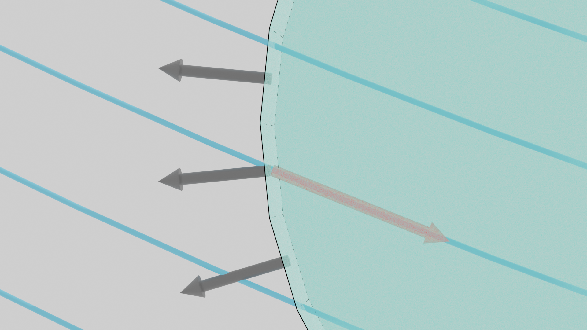
If we consider a small region of outflow from the control surface the fluid will flow along the local streamline. This will be at some angle relative to the local surface normal $\Delta \vec{A}$ of the control volume. The video below shows a cylindrical control volume with exaggerated faces and a number of streamlines showing the flow field as they pass through the control volume. The video highlights the fluid exiting just one of the faces of the control volume and is shown as an extrusion that follows the direction of the local streamline. As the camera reorientates notice how there is an angle $\alpha$ between the velocity vector, which must follow the streamline, and the surface normal $\Delta \vec{A}$ of the control surface. You should be able to visualise similar behaviour for the other outflow faces.
Let's take a look at the last frame of the video. We are highlighting a region of fluid exiting a single face, with area $\Delta A$, normal vector $\Delta \vec{A}$ and velocity $\vec{V}$. The fluid is extruded a length $\Delta l$. The red velocity vector $\vec{V}$ has some angle $\alpha$ relative to the local normal vector on the control surface. The volume of the extruded region of fluid can be calculated from:
\begin{equation*} \Delta \rlap{V}{-} = \Delta l \cos{\alpha} \Delta A \end{equation*}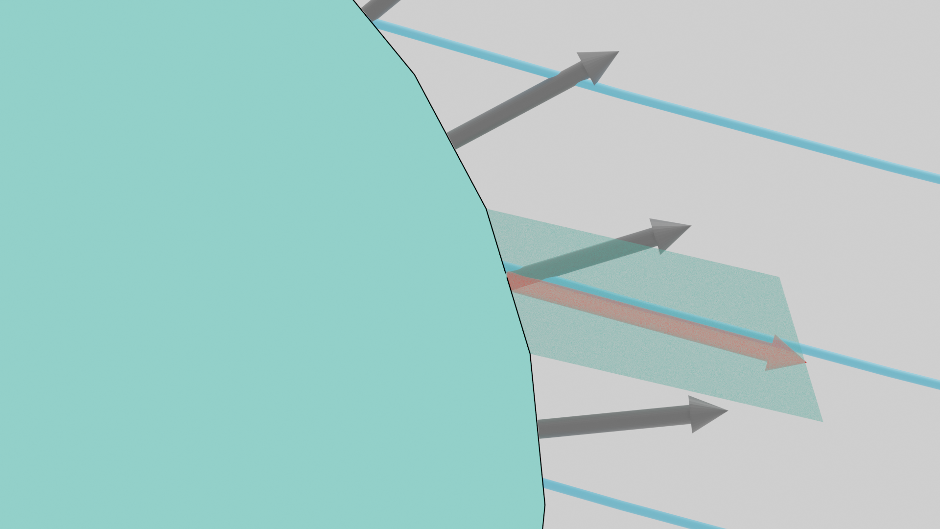
Therefore the amount of property $N$ within this extruded region is:
\begin{equation*} \left( n \rho \delta \rlap{V}{-} \right)_{t_0 + \Delta t} = \left( n \rho \Delta l \cos{\alpha} \Delta A \right)_{t_0 + \Delta t} \end{equation*}As $\Delta A \rightarrow 0$ we can integrate over all the faces of the control surface to obtain the total amount of property $N$ that is transported out of the control volume during time interval $\Delta t$:
\begin{equation*} \left( \int\limits_{III} n \rho \delta \rlap{V}{-} \right)_{t_0 + \Delta t} = \left(~\int\limits_{CS_\text{outflow}} n \rho \Delta l \cos{\alpha} ~ d A \right)_{t_0 + \Delta t} \end{equation*}How would this work at the inflow?
Since the normal vector $\Delta \vec{A}$ always points outward from the control volume the only difference between an inflow and an outflow is the angle $\alpha$.
It is apparent that we can determine if there is inflow or outflow based on the angle $\alpha$.
- outflow if $0 \leq \alpha < \frac{\pi}{2}$
- inflow if $\frac{\pi}{2} \leq \alpha < \pi$
Or in other words if the dot product $\vec{V} \cdot \Delta \vec{A}$ is positive, it is an outflow and if it is negative it is an inflow.
Inflow and outflow can therefore be combined and the integral evaluated over the control surface of the control volume.
\begin{equation*} \lim_{\Delta t \rightarrow 0} \left( \frac{\left(~\int\limits_{III} n \rho d\rlap{V}{-}\right)_{t_0 + \Delta t}}{\Delta t} - \frac{\left(~\int\limits_{I} n \rho d\rlap{V}{-}\right)_{t_0 + \Delta t}}{\Delta t} \right) \approx \lim_{\Delta t \rightarrow 0} \int\limits_{CS} n \rho \frac{\Delta l}{\Delta t} \cos{\alpha}~{dA} \end{equation*}We can simplify further. The extrusion length $\Delta l$ occurs over time $\Delta t$ so that $\left\| \vec{V} \right\| = \frac{\Delta l}{\Delta t}$ and the magnitude of the normal vector is equal to the area of the face.
\begin{equation*} \approx \int\limits_{CS} n \rho \left\| \vec{V} \right\| \left\|d \vec{A} \right\| \cos{\alpha} \end{equation*}And as we showed in the previous notebook the definition of the dot product is: $\vec{V} \cdot d\vec{A} = {\left\| \vec{V} \right\| \left\| d\vec{A} \right\|} \cos{\alpha}$, we obtain
Combining these three results yields the Reynolds Transport Theorem relating the system representation to the control volume representation:
Now we can use Python to explore these ideas in code.
import numpy as np
import matplotlib.pyplot as plt

%matplotlib inline
%config InlineBackend.figure_format = 'retina'

# define x and y ranges
x = np.arange(0, 3.2, 0.1) # from 0 up to 2.1 in steps of 0.125. (note that 2.1 is not included)
y = np.arange(-1.1, 1.1, 0.05)

# Create a grid
X, Y = np.meshgrid(x, y)

# Create a simple flow field using a function that we can reuse later
def vel_field(x):
    u = 2 * np.ones(x.shape)
    v = 0.75 * np.cos(np.pi * x)
    return u, v

u, v = vel_field(X)

# Create a new figure for plotting
fig, ax1 = plt.subplots(figsize=(15,10))

# Control Volume
xc0 = 1.5
yc0 = 0
rc = 0.75

theta_res = 60
theta = np.linspace(0,2*np.pi,theta_res)
xc = xc0 + rc * np.cos(theta)
yc = yc0 + rc * np.sin(theta)

CV = plt.Circle((xc0, yc0), rc, ec='None', fc='b', alpha=0.25)
CS = plt.Circle((xc0, yc0), rc, ec='r', ls='--', fc='None')
ax1.add_patch(CV)
ax1.add_patch(CS)

u_normal = np.cos(theta)
v_normal = np.sin(theta)

u_tangent = np.sin(theta)
v_tangent = -np.cos(theta)

# Plot normal vectors
ax1.quiver(xc, yc, u_normal, v_normal,
           angles='xy',
           scale_units='xy',
           scale=20,
           width=0.0025)

# Plot the flow field
ax1.quiver(X, Y, u, v,
           color='b',
           alpha=0.5,
           angles='xy',
           scale_units='xy',
           scale=20,
           width=0.0025)

plt.xlabel("x")
plt.ylabel("y")
plt.xlim([0, 3])
plt.ylim([-1, 1])
ax1.set_aspect('equal')

# Create a new figure for plotting
fig, ax2 = plt.subplots(figsize=(15,10))

CV = plt.Circle((xc0, yc0), rc, ec='None', fc='b', alpha=0.25)
CS = plt.Circle((xc0, yc0), rc, ec='r', ls='--', fc='None')
ax2.add_patch(CV)
ax2.add_patch(CS)

# Evaulate flow field at control surface using our reusable function
u_CS, v_CS = vel_field(xc)

# Plot flow field
ax2.quiver(X, Y, u, v,
           color='b',
           alpha=0.25,
           angles='xy',
           scale_units='xy',
           scale=20,
           width=0.0025)

# Plot normal vectors
ax2.quiver(xc, yc, u_normal, v_normal,
           angles='xy',
           scale_units='xy',
           scale=20,
           width=0.0025)

# Plot flow field on the control surface
ax2.quiver(xc, yc, u_CS, v_CS,
           color='r',
           angles='xy',
           scale_units='xy',
           scale=20,
           width=0.0025)

plt.xlabel("x")
plt.ylabel("y")
plt.xlim([0, 3])
plt.ylim([-1, 1])
ax2.set_aspect('equal')

# Create a new figure for plotting
fig, ax3 = plt.subplots(figsize=(15,10))

CV = plt.Circle((xc0, yc0), rc, ec='None', fc='b', alpha=0.25)
CS = plt.Circle((xc0, yc0), rc, ec='r', ls='--', fc='None')
ax3.add_patch(CV)
ax3.add_patch(CS)

ind_normal = np.empty((theta_res, 0))
for n in range(theta_res):
    ind_normal = np.append(ind_normal,np.dot([u_CS[n],v_CS[n]],[u_normal[n],v_normal[n]]))

ind_tangent = np.empty((theta_res, 0))
for n in range(theta_res):
    ind_tangent = np.append(ind_tangent,np.dot([u_CS[n],v_CS[n]],[u_tangent[n],v_tangent[n]]))


# Plot flow field
ax3.quiver(X, Y, u, v,  color='b', alpha=0.25, angles='xy', scale_units='xy', scale=15, width=0.0025)

# Plot signed normal vectors to indicate inflow and outflow
ax3.quiver(xc, yc, ind_normal*u_normal, ind_normal*v_normal,
           color='b',
           angles='xy',
           scale_units='xy',
           scale=20,
           width=0.0025)

# Plot signed tangent vectors to indicate inflow and outflow
ax3.quiver(xc, yc, ind_tangent*u_tangent, ind_tangent*v_tangent,
           color='g',
           angles='xy',
           scale_units='xy',
           scale=20,
           width=0.0025)

# Plot flow field on the control surface
ax3.quiver(xc, yc, u_CS, v_CS,
           color='r',
           angles='xy',
           scale_units='xy',
           scale=20,
           width=0.0025)

plt.xlabel("x")
plt.ylabel("y")
plt.xlim([0, 3])
plt.ylim([-1, 1])
ax3.set_aspect('equal')

fig, ax4 = plt.subplots(figsize=(15,10))

mask = np.sqrt((X - xc0)**2 + (Y - yc0)**2)
mask = mask < rc

X_masked = X[mask]
Y_masked = Y[mask]
u_masked = u[mask]
v_masked = v[mask]

start_points = np.stack((xc,yc)).T
in_points  = start_points[ind_normal<0,:]
out_points = start_points[ind_normal>0,:]

plt.plot(in_points[:,0],in_points[:,1],'co')
plt.plot(out_points[:,0],out_points[:,1],'mo')

ax4.streamplot(X, Y, u, v, linewidth=2, start_points=in_points,integration_direction='backward', color='k',broken_streamlines=False)
ax4.streamplot(X, Y, u, v, linewidth=2, start_points=out_points,integration_direction='forward', color='k',broken_streamlines=False)

CV = plt.Circle((xc0, yc0), rc, ec='None', fc='b', alpha=0.25)
CS = plt.Circle((xc0, yc0), rc, ec='r', ls='--', fc='None')
ax4.add_patch(CV)
ax4.add_patch(CS)

# Plot flow field
ax4.quiver(X_masked, Y_masked, u_masked, v_masked,
           color='c',
           angles='xy',
           scale_units='xy',
           scale=20,
           width=0.0025)

# Plot signed normal vectors to indicate inflow and outflow
ax4.quiver(xc, yc, ind_normal*u_normal, ind_normal*v_normal,
           color='b',
           angles='xy',
           scale_units='xy',
           scale=20,
           width=0.0025)

# Plot signed tangent vectors to indicate inflow and outflow
ax4.quiver(xc, yc, ind_tangent*u_tangent, ind_tangent*v_tangent,
           color='g',
           angles='xy',
           scale_units='xy',
           scale=20,
           width=0.0025)

# Plot flow field on the control surface
ax4.quiver(xc, yc, u_CS, v_CS,
           color='r',
           angles='xy',
           scale_units='xy',
           scale=20,
           width=0.0025)

plt.xlabel("x")
plt.ylabel("y")
plt.xlim([0, 3])
plt.ylim([-1, 1])
ax4.set_aspect('equal')

Finishing Up
We have derived the Reynold Transport Theorem and should now understand its importance in allowing us to switch from a Lagrangian to an Eulerian control volume.