Algebra: Quantum Mechanics¶

Reference: http://qutip.org/docs/latest/index.html

Some Facts from Quantum Physics:¶

1. Web function $\psi(x)$ is projection of abstract quantum state $|\psi \rangle $ (in a certain representation) to a position space (representation) basis $|x \rangle$. Where, $|x\rangle$ is a continuous basis with orthogonality relation $\langle x^{'}|x\rangle = \delta(x,x^{'})$.

2. Web function $\phi(p)$ is projection of abstract quantum state $|\psi \rangle $ in a certain representation to a momentum space (representation) basis $|p \rangle$. Where, $|p\rangle$ is a continuous basis with orthogonality relation $\langle p^{'}|p\rangle = \delta(p,p^{'})$.

3. Spherical Harmonics $Y_{l,m}(\theta,\phi)$ is projection of abstract quantum state $| l,m \rangle$ (in angular momnetum representation) to a position space (representation) basis $|\theta, \phi \rangle$.

4. An unitary operator $U$ can be constructed from exponentiation of Hermitian Operator $H$.

One application of this approach is defining Rotation matrix $R$ in Hilbert space by implementation of angular momentum Operator (e.g., $L_x, L_y, L_z$) as generator of rotation in specific irreducible subspace (e.g.,l=0,l=1,l=2...) of the Hilbert space. A general rotation in Hilbert space is infinite dimentional rotation matrix. In eigen basis of anfgular momentum ($L^{2}, L_z$), this matrix appears as block diagonal matrix with block representing rotation in specific irriducible sub-space.

5. In hydrogen like system with spinless particle, operator hamiltonian $H$, square of Angular momentum $L^{2}$ and z-omponent of $L$ operator($L_z$) commute with eachother which means these operators are simultaneously diagonalized. The benefit of of this relation is that once we are able to find eigen basis of $L_z$ operator, we get the eigen basis of Hamiltonian as well. The eighen states of hamiltonian represents the energy level of the system.

1. Hydrogen Atom: Angular Momentum and Spherical Harmonics¶

The matrix element of general angular momnetum operators $J,J_z,J_+,J_-$ are as follows:

One can write a python function to provide a matrix element for an arbitrary operators $J,J_z,J_+,J_-$ , but we dont have to work hard now python package qutip provides us these operators as quantum object Quobj (of kind operators). We will try to play around with some of them.

Spin Angular Momentum $s = 1/2, ms = -1/2, 1/2$¶

Matrix size = 2x2

Experiment 1 :¶

• A generic rotation $ U_n(\theta) = e^{-i \theta n.\sigma} = e^{-i (\theta_x \sigma_x + \theta_y \sigma_y + \theta_z \sigma_z)} $

Note: $ U_n(\theta) = e^{-i \theta n.\sigma} \neq e^{-i (\theta_x \sigma_x)} e^{-i (\theta_y \sigma_y)} e^{-i(\theta_z \sigma_z)} $ since pauli matrices are non-commuting.

• Generic quantum state in ($s =1/2$) subspace: $|\psi \rangle = \alpha |\psi_{1/2}\rangle + \beta |\psi_{-1/2}\rangle$

Non-commuting Matrix exponentials

Let us tast above fact by evaluating generic rotation operator $U_n$ around a arbitrary axix $n$ (i.e., $e^{-i (\theta_x \sigma_x + \theta_y \sigma_y + \theta_z \sigma_z)})$ as U_direct and the product of individual rotation operator (i.e., $ e^{-i (\theta_x \sigma_x)} e^{-i (\theta_y \sigma_y)} e^{-i(\theta_z \sigma_z)}$) as U_prod in the code cells below. We will clearly see that thes two terms are not equal verifying relation $e^{-i \theta n.\sigma} \neq e^{-i (\theta_x \sigma_x)} e^{-i (\theta_y \sigma_y)} e^{-i(\theta_z \sigma_z)}$.

• Calculate $e^{-i (\theta_x \sigma_x + \theta_y \sigma_y + \theta_z \sigma_z)})$ as U_direct

• Calculate $e^{-i (\theta_x \sigma_x)} e^{-i (\theta_y \sigma_y)} e^{-i(\theta_z \sigma_z)}$ as product of three individual rotation as U_prod

• Are U_direct and U_prod same Operators?

Why?

We can see these two operators are not same by implement them in same initial state psi0 vector and observe the final states are not same.

• In fact, both of them are Unitary operators with determinant 1

Angular Momentum $l =1, m = -1,0,1$¶

Matrix size = 3x3

• Do $L_x, L_y$ commute?

• What is matrix element of $L^{2}$ ?

Experiment 2¶

• Rotaion $ R(\theta) = e^{-i \theta n.L} = e^{-i (\theta_x L_x + \theta_y L_y + \theta_z L_z)} $

• Generic quantum state in ($l =0$) subspace: $|\psi \rangle = \alpha |\psi_{10}\rangle + \beta |\psi_{11} \rangle + \gamma |\psi_{1-1} \rangle$

Let us find rotation matrix for subspace (l=1) with different values of $\theta_x, \theta_y, \theta_z$

Mini Assignment:

• Roate a random vector $|\psi \rangle $,i.e. ($|\psi \rangle = \alpha |\psi_{10}\rangle + \beta |\psi_{11} \rangle + \gamma |\psi_{1-1} \rangle)$ by implementing R_prod and R_direct calculated above and compere the final state vectors.

Angular Momentum plus Spin: $l = 3/2, m = -3/2,-1/2,1/2,3/2$¶

Matrix size = 4x4

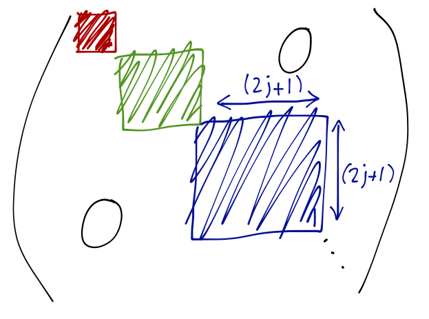
Summary: Rotation in Hilbert Space¶

Structure of a general rotation matrix (R) in Hilbert space

j = 1/2,1,3/2,2,5/2,3,...

• A general rotation matrix ($R$) in hilbert space of basis $|l,m\rangle$ appears as block diagonal matrix, wher every block represents the rotation with specific subspaces called irriducible subspace.
• In the same basis $|l,m\rangle$ Hamiltonian Matrix $H$, $J^2$ and $J_z$ are simultaneously diagonalized.

2. Quantum Harmonic Oscillator¶

3. Random Matrices¶

• Random hermitian matrix

• Random Unitary Matrix

Mini Assignment:¶

1. Generate a random Hermitian matrix $H$ of size 10 by 10.
2. Diagonalize the Hermitian Operator $H$ and find eigne values and eigen vectors.
3. Create a Unitary operator $U$ by exponentiating the Hermitian matrix i.e. $U = e^{-i \alpha H}$.
4. Apply operator $U$ over eigen vectors of operator $H$. Does this operation preserve the norm of eigen vectors?
5. Check that $U$ is unitary or not.
6. What is the determinant of $U$?

Reference¶

1. Rotation
2. Spherical Harmonics
3. Angular Momentum