** DIscBIO: a user-friendly pipeline for biomarker discovery in single-cell transcriptomics**
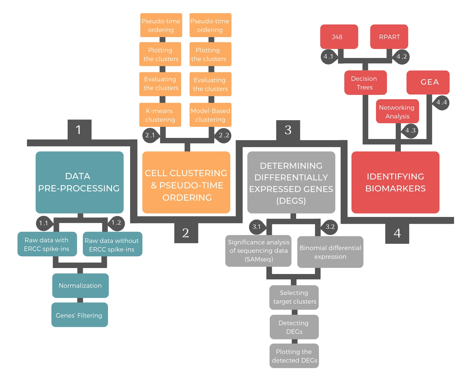
The pipeline consists of four successive steps: data pre-processing, cellular clustering and pseudo-temporal ordering, determining differential expressed genes and identifying biomarkers.
Required Packages
library(DIscBIO)
Loading required package: SingleCellExperiment

Loading required package: SummarizedExperiment

Loading required package: MatrixGenerics

Loading required package: matrixStats


Attaching package: ‘MatrixGenerics’


The following objects are masked from ‘package:matrixStats’:

    colAlls, colAnyNAs, colAnys, colAvgsPerRowSet, colCollapse,
    colCounts, colCummaxs, colCummins, colCumprods, colCumsums,
    colDiffs, colIQRDiffs, colIQRs, colLogSumExps, colMadDiffs,
    colMads, colMaxs, colMeans2, colMedians, colMins, colOrderStats,
    colProds, colQuantiles, colRanges, colRanks, colSdDiffs, colSds,
    colSums2, colTabulates, colVarDiffs, colVars, colWeightedMads,
    colWeightedMeans, colWeightedMedians, colWeightedSds,
    colWeightedVars, rowAlls, rowAnyNAs, rowAnys, rowAvgsPerColSet,
    rowCollapse, rowCounts, rowCummaxs, rowCummins, rowCumprods,
    rowCumsums, rowDiffs, rowIQRDiffs, rowIQRs, rowLogSumExps,
    rowMadDiffs, rowMads, rowMaxs, rowMeans2, rowMedians, rowMins,
    rowOrderStats, rowProds, rowQuantiles, rowRanges, rowRanks,
    rowSdDiffs, rowSds, rowSums2, rowTabulates, rowVarDiffs, rowVars,
    rowWeightedMads, rowWeightedMeans, rowWeightedMedians,
    rowWeightedSds, rowWeightedVars


Loading required package: GenomicRanges

Loading required package: stats4

Loading required package: BiocGenerics

Loading required package: parallel


Attaching package: ‘BiocGenerics’


The following objects are masked from ‘package:parallel’:

    clusterApply, clusterApplyLB, clusterCall, clusterEvalQ,
    clusterExport, clusterMap, parApply, parCapply, parLapply,
    parLapplyLB, parRapply, parSapply, parSapplyLB


The following objects are masked from ‘package:stats’:

    IQR, mad, sd, var, xtabs


The following objects are masked from ‘package:base’:

    anyDuplicated, append, as.data.frame, basename, cbind, colnames,
    dirname, do.call, duplicated, eval, evalq, Filter, Find, get, grep,
    grepl, intersect, is.unsorted, lapply, Map, mapply, match, mget,
    order, paste, pmax, pmax.int, pmin, pmin.int, Position, rank,
    rbind, Reduce, rownames, sapply, setdiff, sort, table, tapply,
    union, unique, unsplit, which.max, which.min


Loading required package: S4Vectors


Attaching package: ‘S4Vectors’


The following object is masked from ‘package:base’:

    expand.grid


Loading required package: IRanges

Loading required package: GenomeInfoDb

Loading required package: Biobase

Welcome to Bioconductor

    Vignettes contain introductory material; view with
    'browseVignettes()'. To cite Bioconductor, see
    'citation("Biobase")', and for packages 'citation("pkgname")'.


Attaching package: ‘Biobase’


The following object is masked from ‘package:MatrixGenerics’:

    rowMedians


The following objects are masked from ‘package:matrixStats’:

    anyMissing, rowMedians
Loading dataset
The "CTCdataset" dataset consisting of single migratory circulating tumor cells (CTCs) collected from patients with breast cancer. Data are available in the GEO database with accession numbers GSE51827, GSE55807, GSE67939, GSE75367, GSE109761, GSE111065 and GSE86978. The dataset should be formatted in a data frame where columns refer to samples and rows refer to genes. We provide here the possibility to load the dataset either as ".csv" or ".rda" extensions.The dataset should be formatted in a data frame where columns refer to samples and rows refer to genes. We provide here the possibility to load the dataset either as ".csv" or ".rda" extensions.
FileName<-"CTCdataset"        # Name of the dataset
#CSV=TRUE                     # If the dataset has ".csv", the user shoud set CSV to TRUE
CSV=FALSE                     # If the dataset has ".rda", the user shoud set CSV to FALSE

if (CSV==TRUE){
    DataSet <- read.csv(file = paste0(FileName,".csv"), sep = ",",header=T)
    rownames(DataSet)<-DataSet[,1]
    DataSet<-DataSet[,-1]
} else{
    load(paste0(FileName,".rda"))
    DataSet<-get(FileName)
}
cat(paste0("The ", FileName," contains:","\n","Genes: ",length(DataSet[,1]),"\n","cells: ",length(DataSet[1,]),"\n"))
The CTCdataset contains:
Genes: 13181
cells: 1462
1. Preparing the dataset
FG<- DISCBIO(DataSet)
FG<-Normalizedata(FG, mintotal=1000, minexpr=0, minnumber=0, maxexpr=Inf, downsample=FALSE, dsn=1, rseed=17000)
FG<-FinalPreprocessing(FG,GeneFlitering="ExpF",export = TRUE)        # The GeneFiltering should be set to "ExpF"

GolgiFragGeneList<- read.csv(file = "GolgiFragGeneList.csv", sep = ",",header=F)
Data<-FG@fdata
genes<-rownames(Data)
gene_list<- GolgiFragGeneList[,1]
idx_genes <- is.element(genes,gene_list)
OAdf<-Data[idx_genes,]
FG@fdata<-OAdf
dim(FG@fdata)
cat(paste0("A list of ", length(OAdf[,1]), " genes will be used for the clustering","\n"))
The gene filtering method = Noise filtering

The Filtered Normalized dataset contains:
Genes: 13181
cells: 1448


The Filtered Normalized dataset was saved as: filteredDataset.Rdata
- 97
- 1448
A list of 97 genes will be used for the clustering
2. Cellular Clustering and Pseudo Time ordering
load("fg.RData")               # Loading the "fg" object that includes the data of the k-means clustering
FG<-fg                         # Storing the data of fg in the FG
########## Removing the unneeded objects
rm(DataSet)
rm(fg)
rm(Data)
rm(OAdf)

plotGap(FG)                                               ### Plotting gap statistics

############ Plotting the clusters
withr::with_options(repr.plot.width=12, repr.plot.height=12)
plottSNE(FG)

FG<-pseudoTimeOrdering(FG,quiet = TRUE, export = FALSE)
plotOrderTsne(FG)

Evaluating the stability and consistancy of the clusters
# Silhouette plot
withr::with_options(repr.plot.width=12, repr.plot.height=25)
plotSilhouette(FG,K=4)       # K is the number of clusters

# Jaccard Plot
withr::with_options(repr.plot.width=12, repr.plot.height=12)
Jaccard(FG,Clustering="K-means", K=4, plot = TRUE)     # Jaccard
- 0.749
- 0.671
- 0.545
- 0.772

Plotting the gene expression of a particular gene in a tSNE map
g='ENSG00000171611'                   #### Plotting the log expression of  PTCRA
plotExptSNE(FG,g)

g='ENSG00000111057'                   #### Plotting the log expression of  KRT18
plotExptSNE(FG,g)
