Notebook

In [2]:

from __future__ import division, print_function
%matplotlib inline
import sys
sys.path.insert(0,'..') # allow us to format the book

# use same formatting as rest of book so that the plots are
# consistant with that look and feel.
import book_format
book_format.load_style('..')

Out[2]:

This notebook creates the animations for the Multivariate Kalman Filter chapter. It is not really intended to be a readable part of the book, but of course you are free to look at the source code, and even modify it. However, if you are interested in running your own animations, I'll point you to the examples subdirectory of the book, which contains a number of python scripts that you can run and modify from an IDE or the command line. This module saves the animations to GIF files, which is quite slow and not very interactive.

In [3]:

import stats
import numpy as np
from matplotlib.patches import Ellipse
import matplotlib.pyplot as plt
from matplotlib import cm
from mpl_toolkits.mplot3d import Axes3D

# this code lets me animate the 3d covariance. to be honest I do not find it
# very instructive or compelling so I am not using it for now.
def plot_3d_covariance(ax, mean, cov):
    """ plots a 2x2 covariance matrix positioned at mean. mean will be plotted
    in x and y, and the probability in the z axis.

    Parameters
    ----------
    mean :  2x1 tuple-like object
        mean for x and y coordinates. For example (2.3, 7.5)

    cov : 2x2 nd.array
       the covariance matrix

    """

    # compute width and height of covariance ellipse so we can choose
    # appropriate ranges for x and y
    o,w,h = stats.covariance_ellipse(cov,3)
    # rotate width and height to x,y axis
    wx = abs(w*np.cos(o) + h*np.sin(o))*1.2
    wy = abs(h*np.cos(o) - w*np.sin(o))*1.2


    # ensure axis are of the same size so everything is plotted with the same
    # scale
    if wx > wy:
        w = wx
    else:
        w = wy

    minx = mean[0] - w
    maxx = mean[0] + w
    miny = mean[1] - w
    maxy = mean[1] + w
    #print (minx, maxx, miny, maxy)
    
    minx = -9.57238091319 
    maxx= 13.5723809132 
    miny = -4.57238091319 
    maxy = 18.5723809132

    xs = np.arange(minx, maxx, (maxx-minx)/40.)
    ys = np.arange(miny, maxy, (maxy-miny)/40.)
    xv, yv = np.meshgrid (xs, ys)

    zs = np.array([100.* stats.multivariate_gaussian(np.array([x,y]),mean,cov) \
                   for x,y in zip(np.ravel(xv), np.ravel(yv))])
    zv = zs.reshape(xv.shape)

    ax.plot_surface(xv, yv, zv, rstride=1, cstride=1, cmap=cm.autumn)

    ax.set_xlabel('X')
    ax.set_ylabel('Y')
    ax.set_zlim([0,10])
    #ax.set_ylim([-5,20])
    #ax.set_xlim([-10,10])

    ax.contour(xv, yv, zv, zdir='x', offset=minx-1, cmap=cm.autumn)
    ax.contour(xv, yv, zv, zdir='y', offset=maxy, cmap=cm.BuGn)

In [4]:

import numpy as np
import mkf_internal
import matplotlib.pyplot as plt
from gif_animate import animate
import stats
def mkf_animate(frame):
    global ax
    plt.cla()
    var = (31-frame) / 3
    plot_3d_covariance(ax, (2,7), np.array([[var,0],[0,4.]]))
    
    
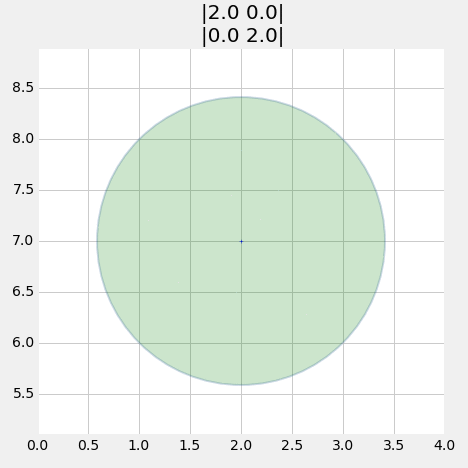
def ellipse_animate(frame):
    
    plt.cla()
    cov = frame/15.
    P = np.array([[2,cov],[cov,2]])
    stats.plot_covariance_ellipse((2,7), cov=P, facecolor='g', alpha=0.2, 
                              title='|2.0 {:.1f}|\n|{:.1f} 2.0|'.format(cov, cov))

fig = plt.figure()
#ax = fig.add_subplot(111, projection='3d')
animate('multivariate_ellipse.gif', ellipse_animate, 30, 125)

<matplotlib.figure.Figure at 0x7effd7d90630>

In [5]:

import numpy as np
from matplotlib.patches import Ellipse
import matplotlib.pyplot as plt
from matplotlib import cm
from mpl_toolkits.mplot3d import Axes3D
from gif_animate import animate
import numpy.random as random
from DogSensor import DogSensor
import stats
from filterpy.common import Q_discrete_white_noise
from filterpy.kalman import KalmanFilter

def dog_tracking_filter(R,Q=0,cov=1.):
    dog_filter = KalmanFilter (dim_x=2, dim_z=1)
    dog_filter.x = np.array([0, 0])   # initial state (location and velocity)
    dog_filter.F = np.array([[1,1],
                             [0,1]])  # state transition matrix
    dog_filter.H = np.array([[1,0]])  # Measurement function
    dog_filter.R *= R                 # measurement uncertainty
    dog_filter.P *= cov               # covariance matrix 
    if np.isscalar(Q):
        dog_filter.Q = Q_discrete_white_noise(2, var=Q)
    else:
        dog_filter.Q = Q
    return dog_filter


R = 5
Q = .01
noise = 2.
P=20.
dog = DogSensor(velocity=1,noise_var=noise)
f = dog_tracking_filter(R=R, Q=Q, cov=P)
random.seed(200)
zs = []
xs = []
def animate_track(frame):
    if frame > 30: return
    
    plt.gca().set_xlim(-100,100)
    if frame == 0:
        stats.plot_covariance_ellipse ((0, f.x[0]), cov=f.P, axis_equal=True, 
                                       facecolor='g', edgecolor=None, alpha=0.2)
        xs.append (f.x[0])
        
    z = dog.sense()
    zs.append(z)
    f.update(z)
    xs.append (f.x[0])
    
    stats.plot_covariance_ellipse ((frame+1, f.x[0]), cov=f.P, axis_equal=True, 
                                       facecolor='g', edgecolor=None, alpha=0.5,
                                       xlim=(-5,30), ylim=(-5,30))
    
    plt.plot(zs, c='r', linestyle='dashed')
    plt.plot(xs, c='b')
    f.predict()

animate('multivariate_track1.gif', animate_track, 37, 200, figsize=(10.5, 10.5))