from IPython.display import Image
from IPython.core.display import HTML
Example 1
Consider the flow of a fluid $A$ that has the following density $\rho$, and a viscosity $\mu$ down a pipe of diamtere $D$ and surface roughness $e$ at a mean flow velocity $V$
Image(url= "https://www.lmnoeng.com/Pressure/Pressure_Drop_dwg.jpg")
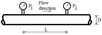
We are measuring the pressure drop in the pipe between two different position $\Delta p = p_2 - p_1$ separated by a distance $L$. $$\Delta p_L = f(V, D, \rho, \mu, L, e)$$
Using Buckingham Pi theorem we can reduce the dimensionality of the problem $$f(V, D, \rho, \mu, L, e) \implies f(\pi_1, \pi_2, \cdots)$$ where $\pi_i$ are dimensionless parameters constructed from the original variables.
from src.buckinghampi import BuckinghamPi
pipe_flow = BuckinghamPi(physical_dimensions='m l t')
pipe_flow.add_variable(name='dp',expression='m/(l*t**2)')
pipe_flow.add_variable(name='V',expression='l/t')
pipe_flow.add_variable(name='D',expression='l')
pipe_flow.add_variable(name='rho',expression='m/(l**3)')
pipe_flow.add_variable(name='L',expression='l')
pipe_flow.add_variable(name='mu',expression='m/(l*t)')
pipe_flow.add_variable(name='e',expression='l')

pipe_flow.generate_pi_terms()

for piterms in pipe_flow.pi_terms:
  print('-----------------')
  for term in piterms:
    print(term)
100%|██████████| 5040/5040 [00:12<00:00, 411.17it/s]
-----------------
L/e
D/e
V*e*rho/mu
dp*e**2*rho/mu**2
-----------------
e/L
L**2*dp*rho/mu**2
D/L
L*V*rho/mu
-----------------
L/e
D/e
mu/(V*e*rho)
dp/(V**2*rho)
-----------------
e/L
D/L
mu/(L*sqrt(dp)*sqrt(rho))
V*sqrt(rho)/sqrt(dp)
-----------------
L/e
D/e
mu/(sqrt(dp)*e*sqrt(rho))
V*sqrt(rho)/sqrt(dp)
-----------------
e/L
dp/(V**2*rho)
mu/(L*V*rho)
D/L
-----------------
L/e
D/e
V*e*rho/mu
dp*e/(V*mu)
-----------------
e/L
D/L
L**2*dp*rho/mu**2
V*mu/(L*dp)
-----------------
D/L
e/L
L*dp/(V*mu)
L*V*rho/mu
-----------------
e/D
L/D
D**2*dp*rho/mu**2
V*mu/(D*dp)
-----------------
e/D
L/D
D*dp/(V*mu)
D*V*rho/mu
-----------------
e/D
L/D
mu/(D*sqrt(dp)*sqrt(rho))
V*sqrt(rho)/sqrt(dp)
-----------------
D/L
e/L
V*mu/(L*dp)
V**2*rho/dp
-----------------
L/D
e/D
V*mu/(D*dp)
V**2*rho/dp
-----------------
D*V*rho/mu
e/D
D**2*dp*rho/mu**2
L/D
-----------------
dp/(V**2*rho)
e/D
mu/(D*V*rho)
L/D
-----------------
V*mu/(dp*e)
L/e
V**2*rho/dp
D/e
-----------------
dp*e/(V*mu)
L*dp/(V*mu)
D*dp/(V*mu)
V**2*rho/dp
-----------------
D*V*rho/mu
V*e*rho/mu
dp/(V**2*rho)
L*V*rho/mu
-----------------
L/e
dp*e**2*rho/mu**2
D/e
V*mu/(dp*e)
-----------------
D*sqrt(dp)*sqrt(rho)/mu
sqrt(dp)*e*sqrt(rho)/mu
V*sqrt(rho)/sqrt(dp)
L*sqrt(dp)*sqrt(rho)/mu
Example 2
The stability of a numerical time integrator in a fluid flow simulation for an incompressible flow on a staggered uniform grid is hinged upon the following set of variables:
- Advection velocity: $u \rightarrow \frac{L}{T}$
- Density of the fluid: $\rho \rightarrow \frac{M}{L**3}$
- Dynamic viscosity: $\mu \rightarrow \frac{M}{LT}$
- Grid spacing: $\mathrm{d}x \rightarrow L$
- Time step: $\mathrm{d}t \rightarrow T$
using the Buckingham Pi module we can obtain the dimensionless $\pi$ terms that describe this example
stability = BuckinghamPi('M L T')
stability.add_variable('u','L/T')
stability.add_variable('rho','M/(L**3)')
stability.add_variable('mu','M/(L*T)')
stability.add_variable('dx','L')
stability.add_variable('dt','T')
stability.generate_pi_terms()

for piterms in stability.pi_terms:
  print('-----------------')
  for term in piterms:
    print(term)
100%|██████████| 120/120 [00:00<00:00, 617.75it/s]
-----------------
dx**2*rho/(dt*mu)
dt*u/dx
-----------------
dx*sqrt(rho)/(sqrt(dt)*sqrt(mu))
sqrt(dt)*sqrt(rho)*u/sqrt(mu)
-----------------
dx/(dt*u)
dt*rho*u**2/mu
-----------------
dx*rho*u/mu
dt*mu/(dx**2*rho)
-----------------
dx*rho*u/mu
dt*u/dx
-----------------
dt*mu/(dx**2*rho)
dt*u/dx
-----------------
dx/(dt*u)
mu/(dt*rho*u**2)
-----------------
mu/(dx*rho*u)
dt*u/dx
-----------------
dt*rho*u**2/mu
dx*rho*u/mu