Overview
1. Baseline Cats vs Dogs Image Classifier (~70% Accuracy)
|___ 1.1. Data
|___ 1.2. Model
|___ 1.3. Training
|___ 1.4. Testing
2. Baseline + Data Augmentation (~73% Accuracy)
|___ 2.1. Data Augmentation
|___ 2.2. Model
|___ 2.3. Training
|___ 2.4. Testing
3. Transfer Learning (~90% Accuracy)
|___ 3.1. Introduction
|___ 3.2. Convolutional layers and Filters
|___ 3.3. Pooling layers
4. Visualizing CNN Learning
1. Baseline Cats vs Dogs Image Classifier
1.1. Data
import warnings
warnings.simplefilter("ignore")
# Import relevant packages
from __future__ import absolute_import, division, print_function # make it compatible w Python 2
import os
import h5py # to handle weights
import os, random
import numpy as np
import pandas as pd
import cv2 #conda install open-cv
import matplotlib.pyplot as plt
%matplotlib inline
from PIL import Image
from tensorflow.keras.models import Sequential
from tensorflow.keras.layers import Input, Dropout, Flatten, Convolution2D, MaxPooling2D, Dense, Activation, ZeroPadding2D
from tensorflow.keras.optimizers import RMSprop
from tensorflow.keras.callbacks import ModelCheckpoint, Callback, EarlyStopping
from tensorflow.keras.preprocessing.image import ImageDataGenerator
from tensorflow.keras.preprocessing.image import array_to_img, img_to_array, load_img
from tensorflow.keras.models import model_from_json
from tensorflow.keras.preprocessing import image
from IPython.display import Image, display
# fix random seed for reproducibility
np.random.seed(150)
# Look at files, note all cat images and dog images are unique
for path, dirs, files in os.walk('./data'):
print('FOLDER',path)
for f in files[:2]:
print(f)
FOLDER ./data FOLDER ./data/test FOLDER ./data/test/catvdog try039.jpg try005.jpg FOLDER ./data/train FOLDER ./data/train/dogs dog0113.jpg dog0675.jpg FOLDER ./data/train/cats cat0852.jpg cat0846.jpg FOLDER ./data/validation FOLDER ./data/validation/dogs dog001275.jpg dog001261.jpg FOLDER ./data/validation/cats cat001138.jpg cat001104.jpg
print('Number of cat training images:', len(next(os.walk('./data/train/cats'))[2]))
print('Number of dog training images:', len(next(os.walk('./data/train/dogs'))[2]))
print('Number of cat validation images:', len(next(os.walk('./data/validation/cats'))[2]))
print('Number of dog validation images:', len(next(os.walk('./data/validation/dogs'))[2]))
print('Number of uncategorized test images:', len(next(os.walk('./data/test/catvdog'))[2]))
# There should be 1000 train cat images, 1000 train dogs,
# 400 validation cats, 400 validation dogs, 100 uncategorized
Number of cat training images: 1000 Number of dog training images: 1000 Number of cat validation images: 400 Number of dog validation images: 400 Number of uncategorized test images: 100
# Define variables
TRAIN_DIR = './data/train/'
VAL_DIR = './data/validation/'
TEST_DIR = './data/test/' #mixed cats and dogs
img_width, img_height = 150, 150
n_train_samples = 2000
n_validation_samples = 800
n_epoch = 20
n_test_samples = 100
Data preprocessing
Data should be formatted into appropriately pre-processed floating point tensors before being fed into our network. Currently, our data is JPEG files, so the steps for getting it into our network are roughly:
- Read the picture files.
- Decode the JPEG content to RBG grids of pixels.
- Convert these into floating point tensors.
- Rescale the pixel values (between 0 and 255) to the [0, 1] interval.
Keras has utilities to take care of these steps automatically.
from tensorflow.keras.preprocessing.image import ImageDataGenerator
# All images will be rescaled by 1./255
train_datagen = ImageDataGenerator(rescale=1./255)
test_datagen = ImageDataGenerator(rescale=1./255)
train_generator = train_datagen.flow_from_directory(
# This is the target directory
TRAIN_DIR,
# All images will be resized to 150x150
target_size=(150, 150),
batch_size=20,
# Since we use binary_crossentropy loss, we need binary labels
class_mode='binary')
validation_generator = test_datagen.flow_from_directory(
VAL_DIR,
target_size=(150, 150),
batch_size=20,
class_mode='binary')
Found 2000 images belonging to 2 classes. Found 800 images belonging to 2 classes.
Let's take a look at the output of one of these generators: it yields batches of 150x150 RGB images (shape (20, 150, 150, 3)) and binary labels (shape (20,)). 20 is the number of samples in each batch (the batch size).
for data_batch, labels_batch in train_generator:
print('data batch shape:', data_batch.shape)
print('labels batch shape:', labels_batch.shape)
break
data batch shape: (20, 150, 150, 3) labels batch shape: (20,)
1.2. Model
The right tool for an image classification job is a convnet, so let's try to train one on our data, as an initial baseline. Very similar to LeNet, as a baseline. Roughly ~75% accuracy. Takes 30mins to train on a CPU.
from tensorflow.keras import layers
from tensorflow.keras import models
model = models.Sequential()
model.add(layers.Conv2D(32, (3, 3), activation='relu',
input_shape=(150, 150, 3)))
model.add(layers.MaxPooling2D((2, 2)))
model.add(layers.Conv2D(64, (3, 3), activation='relu'))
model.add(layers.MaxPooling2D((2, 2)))
model.add(layers.Conv2D(128, (3, 3), activation='relu'))
model.add(layers.MaxPooling2D((2, 2)))
model.add(layers.Conv2D(128, (3, 3), activation='relu'))
model.add(layers.MaxPooling2D((2, 2)))
model.add(layers.Flatten())
model.add(layers.Dense(512, activation='relu'))
model.add(layers.Dense(1, activation='sigmoid'))
model.summary()
Model: "sequential" _________________________________________________________________ Layer (type) Output Shape Param # ================================================================= conv2d (Conv2D) (None, 148, 148, 32) 896 _________________________________________________________________ max_pooling2d (MaxPooling2D) (None, 74, 74, 32) 0 _________________________________________________________________ conv2d_1 (Conv2D) (None, 72, 72, 64) 18496 _________________________________________________________________ max_pooling2d_1 (MaxPooling2 (None, 36, 36, 64) 0 _________________________________________________________________ conv2d_2 (Conv2D) (None, 34, 34, 128) 73856 _________________________________________________________________ max_pooling2d_2 (MaxPooling2 (None, 17, 17, 128) 0 _________________________________________________________________ conv2d_3 (Conv2D) (None, 15, 15, 128) 147584 _________________________________________________________________ max_pooling2d_3 (MaxPooling2 (None, 7, 7, 128) 0 _________________________________________________________________ flatten (Flatten) (None, 6272) 0 _________________________________________________________________ dense (Dense) (None, 512) 3211776 _________________________________________________________________ dense_1 (Dense) (None, 1) 513 ================================================================= Total params: 3,453,121 Trainable params: 3,453,121 Non-trainable params: 0 _________________________________________________________________
from tensorflow.keras import optimizers
model.compile(loss='binary_crossentropy',
optimizer=optimizers.RMSprop(lr=1e-4),
metrics=['acc'])
1.3. Training
Let's fit our model to the data using the generator. We do it using the fit_generator method, the equivalent of fit for data generators like ours. Need to define steps_per_epoch because of generator.
history = model.fit_generator(
train_generator,
steps_per_epoch = 2000//32,
epochs = 30,
validation_data = validation_generator,
validation_steps = 800//32,)
WARNING:tensorflow:From <ipython-input-11-4e55b1ae4082>:6: Model.fit_generator (from tensorflow.python.keras.engine.training) is deprecated and will be removed in a future version.
Instructions for updating:
Please use Model.fit, which supports generators.
WARNING:tensorflow:sample_weight modes were coerced from
...
to
['...']
WARNING:tensorflow:sample_weight modes were coerced from
...
to
['...']
Train for 62 steps, validate for 25 steps
Epoch 1/30
62/62 [==============================] - 21s 332ms/step - loss: 0.6983 - acc: 0.5250 - val_loss: 0.6841 - val_acc: 0.5080
Epoch 2/30
62/62 [==============================] - 15s 239ms/step - loss: 0.6750 - acc: 0.5669 - val_loss: 0.6979 - val_acc: 0.5240
Epoch 3/30
62/62 [==============================] - 15s 241ms/step - loss: 0.6648 - acc: 0.5992 - val_loss: 0.6595 - val_acc: 0.5880
Epoch 4/30
62/62 [==============================] - 15s 245ms/step - loss: 0.6229 - acc: 0.6573 - val_loss: 0.6518 - val_acc: 0.6280
Epoch 5/30
62/62 [==============================] - 15s 242ms/step - loss: 0.6033 - acc: 0.6718 - val_loss: 0.6369 - val_acc: 0.6440
Epoch 6/30
62/62 [==============================] - 15s 244ms/step - loss: 0.5703 - acc: 0.6960 - val_loss: 0.6126 - val_acc: 0.6560
Epoch 7/30
62/62 [==============================] - 15s 245ms/step - loss: 0.5575 - acc: 0.7048 - val_loss: 0.6113 - val_acc: 0.6600
Epoch 8/30
62/62 [==============================] - 15s 248ms/step - loss: 0.5346 - acc: 0.7266 - val_loss: 0.6491 - val_acc: 0.6420
Epoch 9/30
62/62 [==============================] - 15s 248ms/step - loss: 0.5125 - acc: 0.7452 - val_loss: 0.6277 - val_acc: 0.6640
Epoch 10/30
62/62 [==============================] - 16s 253ms/step - loss: 0.5119 - acc: 0.7460 - val_loss: 0.5933 - val_acc: 0.6720
Epoch 11/30
62/62 [==============================] - 16s 251ms/step - loss: 0.5067 - acc: 0.7476 - val_loss: 0.6066 - val_acc: 0.6780
Epoch 12/30
62/62 [==============================] - 16s 251ms/step - loss: 0.4851 - acc: 0.7653 - val_loss: 0.6242 - val_acc: 0.6560
Epoch 13/30
62/62 [==============================] - 16s 252ms/step - loss: 0.4533 - acc: 0.7806 - val_loss: 0.5846 - val_acc: 0.6960
Epoch 14/30
62/62 [==============================] - 16s 250ms/step - loss: 0.4627 - acc: 0.7806 - val_loss: 0.5771 - val_acc: 0.7000
Epoch 15/30
62/62 [==============================] - 15s 250ms/step - loss: 0.4423 - acc: 0.7935 - val_loss: 0.5975 - val_acc: 0.6840
Epoch 16/30
62/62 [==============================] - 16s 252ms/step - loss: 0.4255 - acc: 0.7984 - val_loss: 0.5868 - val_acc: 0.6980
Epoch 17/30
62/62 [==============================] - 16s 252ms/step - loss: 0.4061 - acc: 0.8242 - val_loss: 0.6005 - val_acc: 0.6960
Epoch 18/30
62/62 [==============================] - 16s 253ms/step - loss: 0.3906 - acc: 0.8169 - val_loss: 0.5854 - val_acc: 0.7140
Epoch 19/30
62/62 [==============================] - 16s 253ms/step - loss: 0.3963 - acc: 0.8339 - val_loss: 0.5785 - val_acc: 0.7180
Epoch 20/30
62/62 [==============================] - 16s 253ms/step - loss: 0.3632 - acc: 0.8387 - val_loss: 0.6523 - val_acc: 0.6900
Epoch 21/30
62/62 [==============================] - 16s 253ms/step - loss: 0.3849 - acc: 0.8315 - val_loss: 0.5909 - val_acc: 0.7060
Epoch 22/30
62/62 [==============================] - 16s 252ms/step - loss: 0.3301 - acc: 0.8661 - val_loss: 0.5957 - val_acc: 0.7160
Epoch 23/30
62/62 [==============================] - 16s 252ms/step - loss: 0.3073 - acc: 0.8750 - val_loss: 0.6609 - val_acc: 0.7100
Epoch 24/30
62/62 [==============================] - 16s 252ms/step - loss: 0.3093 - acc: 0.8605 - val_loss: 0.5904 - val_acc: 0.7180
Epoch 25/30
62/62 [==============================] - 15s 250ms/step - loss: 0.3074 - acc: 0.8742 - val_loss: 0.6206 - val_acc: 0.7160
Epoch 26/30
62/62 [==============================] - 16s 252ms/step - loss: 0.2893 - acc: 0.8798 - val_loss: 0.6226 - val_acc: 0.7120
Epoch 27/30
62/62 [==============================] - 16s 255ms/step - loss: 0.2874 - acc: 0.8806 - val_loss: 0.6970 - val_acc: 0.7020
Epoch 28/30
62/62 [==============================] - 16s 257ms/step - loss: 0.2549 - acc: 0.9048 - val_loss: 0.8155 - val_acc: 0.6840
Epoch 29/30
62/62 [==============================] - 16s 260ms/step - loss: 0.2433 - acc: 0.9089 - val_loss: 0.6744 - val_acc: 0.7240
Epoch 30/30
62/62 [==============================] - 16s 256ms/step - loss: 0.2432 - acc: 0.9073 - val_loss: 0.6803 - val_acc: 0.6960
Saving the trained model as .h5 file
model.save('cats_and_dogs_small_1.h5')
Loading a saved .h5 model
from tensorflow.keras.models import load_model
mod = load_model('cats_and_dogs_small_1.h5')
mod.summary() # As a reminder.
Model: "sequential" _________________________________________________________________ Layer (type) Output Shape Param # ================================================================= conv2d (Conv2D) (None, 148, 148, 32) 896 _________________________________________________________________ max_pooling2d (MaxPooling2D) (None, 74, 74, 32) 0 _________________________________________________________________ conv2d_1 (Conv2D) (None, 72, 72, 64) 18496 _________________________________________________________________ max_pooling2d_1 (MaxPooling2 (None, 36, 36, 64) 0 _________________________________________________________________ conv2d_2 (Conv2D) (None, 34, 34, 128) 73856 _________________________________________________________________ max_pooling2d_2 (MaxPooling2 (None, 17, 17, 128) 0 _________________________________________________________________ conv2d_3 (Conv2D) (None, 15, 15, 128) 147584 _________________________________________________________________ max_pooling2d_3 (MaxPooling2 (None, 7, 7, 128) 0 _________________________________________________________________ flatten (Flatten) (None, 6272) 0 _________________________________________________________________ dense (Dense) (None, 512) 3211776 _________________________________________________________________ dense_1 (Dense) (None, 1) 513 ================================================================= Total params: 3,453,121 Trainable params: 3,453,121 Non-trainable params: 0 _________________________________________________________________
1.4. Testing
mod.evaluate(validation_generator,steps=40,verbose=1)[1]
WARNING:tensorflow:sample_weight modes were coerced from
...
to
['...']
40/40 [==============================] - 4s 109ms/step - loss: 0.6621 - acc: 0.7013
0.70125
import matplotlib.pyplot as plt
#history = history_scratch
acc = history.history['acc']
val_acc = history.history['val_acc']
loss = history.history['loss']
val_loss = history.history['val_loss']
epochs = range(len(acc))
plt.plot(epochs, acc, 'bo', label='Training acc')
plt.plot(epochs, val_acc, 'b', label='Validation acc')
plt.title('Training and validation accuracy')
plt.legend()
plt.figure()
plt.plot(epochs, loss, 'bo', label='Training loss')
plt.plot(epochs, val_loss, 'b', label='Validation loss')
plt.title('Training and validation loss')
plt.legend()
plt.show()


These plots are characteristic of overfitting. Our training accuracy increases until it reaches nearly 100%, while our validation accuracy stalls at 70-72%.
Because we only have relatively few training samples (2000), overfitting is going to be our number one concern.
Overfitting can be mitigated using dropout and weight decay (L2 regularization). We are now going to introduce a new one, specific to computer vision, and used almost universally when processing images with deep learning models: Data Augmentation.
2. Baseline + Data augmentation
2.1. Data Augmentation
Overfitting is caused by having too few samples to learn from, rendering us unable to train a model able to generalize to new data. Given infinite data, our model would be exposed to every possible aspect of the data distribution at hand: we would never overfit.
Data augmentation takes the approach of generating more training data from existing training samples, by "augmenting" the samples via a number of random transformations that yield believable-looking images. The goal is that at training time, our model would never see the exact same picture twice. This helps the model get exposed to more aspects of the data and generalize better.
Since we only have few examples, our number one concern should be overfitting. Overfitting happens when a model exposed to too few examples learns patterns that do not generalize to new data, i.e. when the model starts using irrelevant features for making predictions.
# Import image data generator
datagen = ImageDataGenerator(
rotation_range=40, #rotation_range degrees (0-180), range that randomly rotate pictures
width_shift_range=0.2, #width_shift range (fraction of total width) within which to randomly translate pic
height_shift_range=0.2, # -ii-
#rescale value we multiply the data before any other processing.
#Our original images consist in RGB coefficients in the 0-255,
#but such values would be too high for our models to process (given typical learning rate),
# so we target values between 0 and 1 instead by scaling with a 1/255. factor.
rescale=1./255,
#randomly applying shearing transformations (shear mapping is a linear map that
#displaces each point in fixed direction, by an amount proportional to its
#signed distance from a line that is parallel to that direction)
shear_range=0.2,
zoom_range=0.2, #randomly zooming inside pictures
#is for randomly flipping half of the images horizontally
#--relevant when there are no assumptions of horizontal assymetry (e.g. real-world pictures).
horizontal_flip=True,
#is the strategy used for filling in newly created pixels,
#which can appear after a rotation or a width/height shift.
fill_mode='nearest')
Now let's start generating some pictures using this tool and save them to a temporary directory, so we can get a feel for what our augmentation strategy is doing --we disable rescaling in this case to keep the images displayable:
import cv2
img = load_img(TRAIN_DIR+'cats/cat0002.jpg') # this is a PIL image
x = img_to_array(img) # this is a Numpy array with shape (3, 150, 150)
x = x.reshape((1,) + x.shape) # this is a Numpy array with shape (1, 3, 150, 150)
# the .flow() command below generates batches of randomly transformed images
# and saves the results to the `preview/` directory
i = 0
from PIL import Image
if not os.path.exists('preview'):
os.makedirs('preview')
for batch in datagen.flow(x, batch_size=1,
save_to_dir='preview', save_prefix='cat', save_format='jpeg'):
i += 1
if i > 20:
break # otherwise the generator would loop indefinitely
prev_files = next(os.walk('./preview'))[2]
print(prev_files[:4])
def read_image(file_path):
# For image visualization
im = np.array(Image.open(file_path))
img = cv2.imread(file_path, cv2.IMREAD_COLOR) #cv2.IMREAD_GRAYSCALE
return im
def plot_pic(img):
# Plot openCV pic
pic = read_image(img)
plt.figure(figsize=(5,5))
plt.imshow(pic)
plt.show()
for img in prev_files[:10]:
print('Image '+img)
plot_pic('./preview/'+img)
['cat_0_8086.jpeg', 'cat_0_2798.jpeg', 'cat_0_6000.jpeg', 'cat_0_4139.jpeg'] Image cat_0_8086.jpeg

Image cat_0_2798.jpeg

Image cat_0_6000.jpeg

Image cat_0_4139.jpeg

Image cat_0_9567.jpeg

Image cat_0_1507.jpeg

Image cat_0_366.jpeg

Image cat_0_8422.jpeg

Image cat_0_9291.jpeg

Image cat_0_805.jpeg

train_datagen = ImageDataGenerator(
rescale=1./255,
rotation_range=40,
width_shift_range=0.2,
height_shift_range=0.2,
shear_range=0.2,
zoom_range=0.2,
horizontal_flip=True)
# Note that the validation data should not be augmented!
test_datagen = ImageDataGenerator(rescale=1./255)
train_generator = train_datagen.flow_from_directory(
# This is the target directory
TRAIN_DIR,
# All images will be resized to 150x150
target_size=(150, 150),
batch_size=32,
# Since we use binary_crossentropy loss, we need binary labels
class_mode='binary')
validation_generator = test_datagen.flow_from_directory(
VAL_DIR,
target_size=(150, 150),
batch_size=32,
class_mode='binary')
Found 2000 images belonging to 2 classes. Found 800 images belonging to 2 classes.
2.2. Model
# model construction
model = models.Sequential()
model.add(layers.Conv2D(32, (3, 3), activation='relu',
input_shape=(150, 150, 3)))
model.add(layers.MaxPooling2D((2, 2)))
model.add(layers.Conv2D(64, (3, 3), activation='relu'))
model.add(layers.MaxPooling2D((2, 2)))
model.add(layers.Conv2D(128, (3, 3), activation='relu'))
model.add(layers.MaxPooling2D((2, 2)))
model.add(layers.Conv2D(128, (3, 3), activation='relu'))
model.add(layers.MaxPooling2D((2, 2)))
'''
On top of it we stick two fully-connected layers.
We end the model with a single unit and a sigmoid activation, which is perfect for a binary classification.
To go with it we will also use the binary_crossentropy loss to train our model.
'''
model.add(layers.Flatten())
model.add(layers.Dropout(0.5))
model.add(layers.Dense(512, activation='relu'))
model.add(layers.Dense(1, activation='sigmoid'))
model.compile(loss='binary_crossentropy',
optimizer=optimizers.RMSprop(lr=1e-4),
metrics=['acc'])
2.3. Training
history = model.fit_generator(
train_generator,
steps_per_epoch=2000//32,
epochs=50,
validation_data=validation_generator,
validation_steps=800//32,)
WARNING:tensorflow:sample_weight modes were coerced from
...
to
['...']
WARNING:tensorflow:sample_weight modes were coerced from
...
to
['...']
Train for 62 steps, validate for 25 steps
Epoch 1/50
62/62 [==============================] - 33s 534ms/step - loss: 0.6934 - acc: 0.5056 - val_loss: 0.6873 - val_acc: 0.5000
Epoch 2/50
62/62 [==============================] - 26s 414ms/step - loss: 0.6867 - acc: 0.5320 - val_loss: 0.6716 - val_acc: 0.5850
Epoch 3/50
62/62 [==============================] - 25s 410ms/step - loss: 0.6795 - acc: 0.5686 - val_loss: 0.6627 - val_acc: 0.6125
Epoch 4/50
62/62 [==============================] - 26s 413ms/step - loss: 0.6708 - acc: 0.5940 - val_loss: 0.6615 - val_acc: 0.5800
Epoch 5/50
62/62 [==============================] - 25s 411ms/step - loss: 0.6584 - acc: 0.6113 - val_loss: 0.6381 - val_acc: 0.6288
Epoch 6/50
62/62 [==============================] - 26s 415ms/step - loss: 0.6498 - acc: 0.6184 - val_loss: 0.6227 - val_acc: 0.6388
Epoch 7/50
62/62 [==============================] - 25s 411ms/step - loss: 0.6350 - acc: 0.6372 - val_loss: 0.6326 - val_acc: 0.6313
Epoch 8/50
62/62 [==============================] - 25s 406ms/step - loss: 0.6210 - acc: 0.6621 - val_loss: 0.6068 - val_acc: 0.6575
Epoch 9/50
62/62 [==============================] - 26s 415ms/step - loss: 0.6217 - acc: 0.6529 - val_loss: 0.5981 - val_acc: 0.6725
Epoch 10/50
62/62 [==============================] - 25s 408ms/step - loss: 0.6005 - acc: 0.6728 - val_loss: 0.6272 - val_acc: 0.6450
Epoch 11/50
62/62 [==============================] - 26s 415ms/step - loss: 0.6029 - acc: 0.6672 - val_loss: 0.5686 - val_acc: 0.6975
Epoch 12/50
62/62 [==============================] - 26s 414ms/step - loss: 0.5832 - acc: 0.6890 - val_loss: 0.5597 - val_acc: 0.7025
Epoch 13/50
62/62 [==============================] - 26s 419ms/step - loss: 0.5805 - acc: 0.6961 - val_loss: 0.5482 - val_acc: 0.7175
Epoch 14/50
62/62 [==============================] - 26s 412ms/step - loss: 0.5767 - acc: 0.6916 - val_loss: 0.5725 - val_acc: 0.6988
Epoch 15/50
62/62 [==============================] - 26s 413ms/step - loss: 0.5764 - acc: 0.6956 - val_loss: 0.5369 - val_acc: 0.7337
Epoch 16/50
62/62 [==============================] - 26s 421ms/step - loss: 0.5688 - acc: 0.7063 - val_loss: 0.5713 - val_acc: 0.6975
Epoch 17/50
62/62 [==============================] - 26s 426ms/step - loss: 0.5685 - acc: 0.7022 - val_loss: 0.5437 - val_acc: 0.7237
Epoch 18/50
62/62 [==============================] - 27s 430ms/step - loss: 0.5666 - acc: 0.6921 - val_loss: 0.5399 - val_acc: 0.7237
Epoch 19/50
62/62 [==============================] - 27s 434ms/step - loss: 0.5627 - acc: 0.7007 - val_loss: 0.5450 - val_acc: 0.7175
Epoch 20/50
62/62 [==============================] - 26s 427ms/step - loss: 0.5632 - acc: 0.6992 - val_loss: 0.5246 - val_acc: 0.7212
Epoch 21/50
62/62 [==============================] - 27s 431ms/step - loss: 0.5471 - acc: 0.7190 - val_loss: 0.5326 - val_acc: 0.7262
Epoch 22/50
62/62 [==============================] - 27s 433ms/step - loss: 0.5566 - acc: 0.7160 - val_loss: 0.5491 - val_acc: 0.7262
Epoch 23/50
62/62 [==============================] - 27s 429ms/step - loss: 0.5440 - acc: 0.7348 - val_loss: 0.5152 - val_acc: 0.7387
Epoch 24/50
62/62 [==============================] - 27s 430ms/step - loss: 0.5417 - acc: 0.7210 - val_loss: 0.5286 - val_acc: 0.7262
Epoch 25/50
62/62 [==============================] - 27s 436ms/step - loss: 0.5483 - acc: 0.7160 - val_loss: 0.5218 - val_acc: 0.7425
Epoch 26/50
62/62 [==============================] - 27s 435ms/step - loss: 0.5340 - acc: 0.7287 - val_loss: 0.5186 - val_acc: 0.7462
Epoch 27/50
62/62 [==============================] - 27s 437ms/step - loss: 0.5413 - acc: 0.7276 - val_loss: 0.5022 - val_acc: 0.7500
Epoch 28/50
62/62 [==============================] - 27s 436ms/step - loss: 0.5376 - acc: 0.7180 - val_loss: 0.5173 - val_acc: 0.7325
Epoch 29/50
62/62 [==============================] - 27s 441ms/step - loss: 0.5209 - acc: 0.7399 - val_loss: 0.5372 - val_acc: 0.7237
Epoch 30/50
62/62 [==============================] - 27s 435ms/step - loss: 0.5282 - acc: 0.7297 - val_loss: 0.5294 - val_acc: 0.7362
Epoch 31/50
62/62 [==============================] - 27s 439ms/step - loss: 0.5250 - acc: 0.7327 - val_loss: 0.5716 - val_acc: 0.7000
Epoch 32/50
62/62 [==============================] - 27s 440ms/step - loss: 0.5140 - acc: 0.7403 - val_loss: 0.5486 - val_acc: 0.7163
Epoch 33/50
62/62 [==============================] - 28s 445ms/step - loss: 0.5302 - acc: 0.7337 - val_loss: 0.4986 - val_acc: 0.7513
Epoch 34/50
62/62 [==============================] - 27s 438ms/step - loss: 0.5212 - acc: 0.7312 - val_loss: 0.5225 - val_acc: 0.7375
Epoch 35/50
62/62 [==============================] - 26s 418ms/step - loss: 0.5150 - acc: 0.7429 - val_loss: 0.4942 - val_acc: 0.7538
Epoch 36/50
62/62 [==============================] - 26s 424ms/step - loss: 0.5036 - acc: 0.7515 - val_loss: 0.5620 - val_acc: 0.7175
Epoch 37/50
62/62 [==============================] - 26s 427ms/step - loss: 0.5187 - acc: 0.7434 - val_loss: 0.6139 - val_acc: 0.6862
Epoch 38/50
62/62 [==============================] - 26s 418ms/step - loss: 0.5073 - acc: 0.7556 - val_loss: 0.4784 - val_acc: 0.7713
Epoch 39/50
62/62 [==============================] - 26s 421ms/step - loss: 0.5155 - acc: 0.7398 - val_loss: 0.5102 - val_acc: 0.7663
Epoch 40/50
62/62 [==============================] - 26s 416ms/step - loss: 0.4947 - acc: 0.7551 - val_loss: 0.5951 - val_acc: 0.7113
Epoch 41/50
62/62 [==============================] - 26s 425ms/step - loss: 0.5010 - acc: 0.7546 - val_loss: 0.4855 - val_acc: 0.7538
Epoch 42/50
62/62 [==============================] - 27s 428ms/step - loss: 0.5108 - acc: 0.7490 - val_loss: 0.4795 - val_acc: 0.7600
Epoch 43/50
62/62 [==============================] - 26s 414ms/step - loss: 0.5088 - acc: 0.7470 - val_loss: 0.4878 - val_acc: 0.7400
Epoch 44/50
62/62 [==============================] - 26s 427ms/step - loss: 0.4907 - acc: 0.7576 - val_loss: 0.5404 - val_acc: 0.7150
Epoch 45/50
62/62 [==============================] - 26s 425ms/step - loss: 0.4987 - acc: 0.7525 - val_loss: 0.4670 - val_acc: 0.7663
Epoch 46/50
62/62 [==============================] - 26s 418ms/step - loss: 0.4949 - acc: 0.7530 - val_loss: 0.4543 - val_acc: 0.7800
Epoch 47/50
62/62 [==============================] - 27s 429ms/step - loss: 0.4874 - acc: 0.7708 - val_loss: 0.4567 - val_acc: 0.7725
Epoch 48/50
62/62 [==============================] - 27s 436ms/step - loss: 0.4935 - acc: 0.7581 - val_loss: 0.4765 - val_acc: 0.7600
Epoch 49/50
62/62 [==============================] - 29s 463ms/step - loss: 0.4827 - acc: 0.7729 - val_loss: 0.4764 - val_acc: 0.7675
Epoch 50/50
62/62 [==============================] - 28s 458ms/step - loss: 0.4880 - acc: 0.7602 - val_loss: 0.4646 - val_acc: 0.7887
Save the model
model.save('cats_and_dogs_small_1.h5')
Load the model
from keras.models import load_model
mod = load_model('cats_and_dogs_small_2.h5')
mod.summary() # As a reminder.
Using TensorFlow backend.
Model: "sequential_1" _________________________________________________________________ Layer (type) Output Shape Param # ================================================================= conv2d_5 (Conv2D) (None, 148, 148, 32) 896 _________________________________________________________________ max_pooling2d_5 (MaxPooling2 (None, 74, 74, 32) 0 _________________________________________________________________ conv2d_6 (Conv2D) (None, 72, 72, 64) 18496 _________________________________________________________________ max_pooling2d_6 (MaxPooling2 (None, 36, 36, 64) 0 _________________________________________________________________ conv2d_7 (Conv2D) (None, 34, 34, 128) 73856 _________________________________________________________________ max_pooling2d_7 (MaxPooling2 (None, 17, 17, 128) 0 _________________________________________________________________ conv2d_8 (Conv2D) (None, 15, 15, 128) 147584 _________________________________________________________________ max_pooling2d_8 (MaxPooling2 (None, 7, 7, 128) 0 _________________________________________________________________ flatten_2 (Flatten) (None, 6272) 0 _________________________________________________________________ dropout_1 (Dropout) (None, 6272) 0 _________________________________________________________________ dense_3 (Dense) (None, 512) 3211776 _________________________________________________________________ dense_4 (Dense) (None, 1) 513 ================================================================= Total params: 3,453,121 Trainable params: 3,453,121 Non-trainable params: 0 _________________________________________________________________
2.4. Testing
model.evaluate(validation_generator,steps=validation_generator.n//32,verbose=1)[0]
WARNING:tensorflow:sample_weight modes were coerced from
...
to
['...']
25/25 [==============================] - 4s 156ms/step - loss: 0.4646 - acc: 0.7887
0.4646056342124939
acc = history.history['acc']
val_acc = history.history['val_acc']
loss = history.history['loss']
val_loss = history.history['val_loss']
epochs = range(len(acc))
plt.plot(epochs, acc, 'bo', label='Training acc')
plt.plot(epochs, val_acc, 'b', label='Validation acc')
plt.title('Training and validation accuracy')
plt.legend()
plt.figure()
plt.plot(epochs, loss, 'bo', label='Training loss')
plt.plot(epochs, val_loss, 'b', label='Validation loss')
plt.title('Training and validation loss')
plt.legend()
plt.show()


# Plot picture and print class prediction on cats vs dogs (unsorted)
try_images = [TEST_DIR+'catvdog/'+img for img in os.listdir(TEST_DIR+'catvdog/')]
def predict(mod,i=0,r=None):
if r==None:
r=[i]
for idx in r:
if 'DS_Store' in try_images[idx]:
continue
img_path = try_images[idx]
img = image.load_img(img_path, target_size=(150, 150))
x = image.img_to_array(img)
x = np.expand_dims(x, axis=0)
class_pred = mod.predict_classes(x,verbose=0)
if class_pred == 0:
class_guess='CAT'
else:
class_guess='DOG'
print('\n\nI think this is a ' + class_guess)
plot_pic(try_images[idx])
predict(mod,r=range(10))
I think this is a DOG

I think this is a DOG

I think this is a DOG

I think this is a DOG

I think this is a CAT

I think this is a DOG

I think this is a CAT

I think this is a DOG

I think this is a DOG

I think this is a DOG

3. Transfer Learning
3.1. Introduction
Build a more powerful Cats vs Dogs binary classifier
Now we will use Transfer learning and remove the top layer of a pretrained network (VGG16 on Imagenet), extracting the features of the training and validation images and then just training the fully connected top layer of that network. This way we will be able to make accurate predictions even though we just have a small data set.
The data conists of 2000 training images (1000 cats and 1000 dogs), 800 validation images (400 cats and 400 dogs), and 100 test images (cats and dogs mixed). Get the data here.
The pretrained VGG16 weighs that you should load into your model (in order to extract the bottleneck features) can be downloaded here. Extracted features are included so that you can run the code instantly.
The reason why we are using a pretrained network, extracting bottleneck features and training only the top layers is that this is a great way to obtain a high prediction accuracy without having a huge data set and without having to run the training for a long time. It would require much more data and take up to several days to run this analysis and training your own CNN on a personal computer (in order to obtain the same level of accuracy).
3.2. Extract bottleneck features from the data set
A good explanation on how this works (rewritten from source: https://blog.keras.io/building-powerful-image-classification-models-using-very-little-data.html)
Using the bottleneck features of a pre-trained network: 90% accuracy in 1 min (GPU) / 10 mins (CPU)
We are leveraging the predictive power of a network pre-trained on a large dataset. Such a network would have already learned features that are useful for most computer vision problems, and leveraging such features would allow us to reach a better accuracy than any method that would only rely on the available data.
We will use the VGG16 architecture, pre-trained on the ImageNet dataset. Because the ImageNet dataset contains several "cat" classes (persian cat, siamese cat...) and many "dog" classes among its total of 1000 classes, this model will already have learned features that are relevant to our classification problem. In fact, it is possible that merely recording the softmax predictions of the model over our data rather than the bottleneck features would be enough to solve our dogs vs. cats classification problem extremely well. The method presented here is more likely to generalize well to a broader range of problems, including problems featuring classes absent from ImageNet.
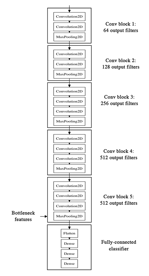
Here's what the VGG16 architecture looks like:
Horizontal visualization

Strategy to extract bottleneck features:
We will only instantiate the convolutional part of the model, everything up to the fully-connected layers. We will pass our training, validation, and test data through this model once, recording the output (the "bottleneck features" from the VGG16 model, ie the output of the last activation maps before the fully-connected layers).
The output will be saved as three numpy arrays, and stored on disk as .npy files.. The reason why we are storing the features offline rather than adding our fully-connected model directly on top of a frozen convolutional base and running the whole thing, is computational effiency. Running VGG16 is expensive, especially if you're working on CPU, and we want to only do it once.
This is how the VGG16 net looks in code
You can see the full implementation here of the network we're building and loading in: https://github.com/fchollet/keras/blob/master/keras/applications/vgg16.py
# VGG 16 model architecture
model = Sequential()
model.add(ZeroPadding2D((1, 1), input_shape=(img_width, img_height, 3)))
model.add(Convolution2D(64, 3, 3, activation='relu', name='conv1_1'))
model.add(ZeroPadding2D((1, 1)))
model.add(Convolution2D(64, 3, 3, activation='relu', name='conv1_2'))
model.add(MaxPooling2D((2, 2), strides=(2, 2)))
model.add(ZeroPadding2D((1, 1)))
model.add(Convolution2D(128, 3, 3, activation='relu', name='conv2_1'))
model.add(ZeroPadding2D((1, 1)))
model.add(Convolution2D(128, 3, 3, activation='relu', name='conv2_2'))
model.add(MaxPooling2D((2, 2), strides=(2, 2)))
model.add(ZeroPadding2D((1, 1)))
model.add(Convolution2D(256, 3, 3, activation='relu', name='conv3_1'))
model.add(ZeroPadding2D((1, 1)))
model.add(Convolution2D(256, 3, 3, activation='relu', name='conv3_2'))
model.add(ZeroPadding2D((1, 1)))
model.add(Convolution2D(256, 3, 3, activation='relu', name='conv3_3'))
model.add(MaxPooling2D((2, 2), strides=(2, 2)))
model.add(ZeroPadding2D((1, 1)))
model.add(Convolution2D(512, 3, 3, activation='relu', name='conv4_1'))
model.add(ZeroPadding2D((1, 1)))
model.add(Convolution2D(512, 3, 3, activation='relu', name='conv4_2'))
model.add(ZeroPadding2D((1, 1)))
model.add(Convolution2D(512, 3, 3, activation='relu', name='conv4_3'))
model.add(MaxPooling2D((2, 2), strides=(2, 2)))
model.add(ZeroPadding2D((1, 1)))
model.add(Convolution2D(512, 3, 3, activation='relu', name='conv5_1'))
model.add(ZeroPadding2D((1, 1)))
model.add(Convolution2D(512, 3, 3, activation='relu', name='conv5_2'))
model.add(ZeroPadding2D((1, 1)))
model.add(Convolution2D(512, 3, 3, activation='relu', name='conv5_3'))
model.add(MaxPooling2D((2, 2), strides=(2, 2)))
# Classification block
model.add(Flatten(name='flatten')(x))
model.add(Dense(4096, activation='relu', name='fc1')(x))
model.add(Dense(4096, activation='relu', name='fc2')(x))
model.add(Dense(classes, activation='softmax', name='predictions')(x))
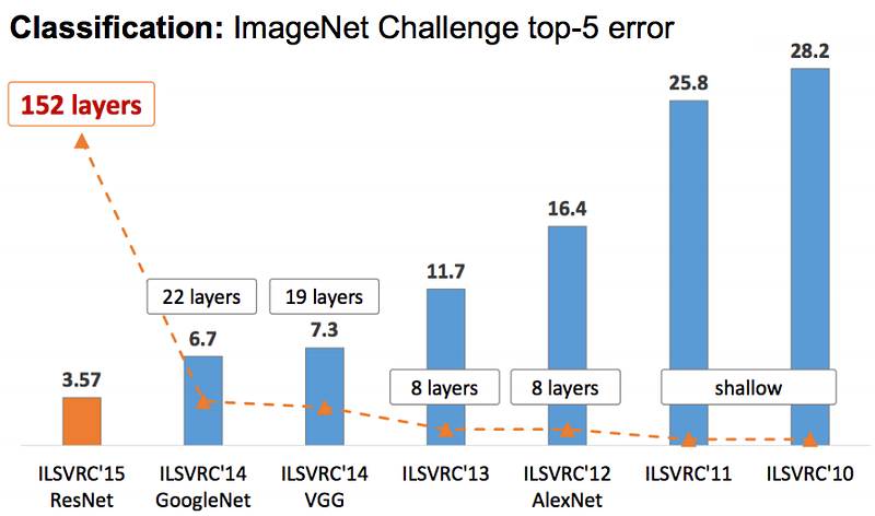
IMAGEnet Benchmarks (the structure we're using today, 2nd place in 2014)
# Function for saving bottleneck features
# This can take ~10mins to run
# Run model once to record the bottleneck features using image data generators:
def save_bottleneck_features():
from tensorflow.keras import applications
model = applications.vgg16.VGG16(include_top=False, weights='imagenet', \
input_tensor=None, input_shape=(img_width, img_height,3))
# documentation: https://keras.io/applications/#vgg16
print('TensorFlow VGG16 model architecture loaded')
# include_top = False, because we drop last layer, then we also only need to
# download weight file that is small
# input_shape with channels last for tensorflow
# Our original images consist in RGB coefficients in the 0-255 interval,
# but such values would be too high for our models to process (given typical learning rate),
# so we target values between 0 and 1 instead by scaling with a 1/255. factor.
datagen = ImageDataGenerator(rescale=1./255)
def generate_features(DIR,n_samples,name_str):
'''This is a generator that will read pictures found in
subfolers of 'data/*', and indefinitely generate
batches of rescaled images used to predict
the bottleneck features of the images once
using model.predict_generator(**args**)'''
print('Generate '+name_str+' image features')
generator = datagen.flow_from_directory(
DIR,
target_size=(img_width, img_height),
batch_size=1,
class_mode=None, # this means our generator will only yield batches of data, no labels
shuffle=False) # our data will be in order, so all first 1000 images will be cats, then 1000 dogs
features = model.predict_generator(generator, n_samples,verbose=True)
# the predict_generator method returns the output of a model, given
# a generator that yields batches of numpy data
np.save('features_'+name_str+'.npy', features) # save bottleneck features to file
generate_features(TEST_DIR, n_test_samples, 'test')
#generate_features(TRAIN_DIR, n_train_samples, 'train')
#generate_features(VAL_DIR, n_validation_samples, 'validation')
print('\nDone! Bottleneck features have been saved')
print('This has been done before the lecture! Takes 5+ mins to run.')
save_bottleneck_features()
This has been done before the lecture! Takes 5+ mins to run. TensorFlow VGG16 model architecture loaded Generate test image features Found 100 images belonging to 1 classes. WARNING:tensorflow:From <ipython-input-26-cc9fde1bd17b>:41: Model.predict_generator (from tensorflow.python.keras.engine.training) is deprecated and will be removed in a future version. Instructions for updating: Please use Model.predict, which supports generators. 100/100 [==============================] - 9s 88ms/step Done! Bottleneck features have been saved
# Extra
# Obtain class labels and binary classification for validation data
datagen = ImageDataGenerator(rescale=1./255)
val_gen = datagen.flow_from_directory(VAL_DIR,target_size=(img_width, img_height),
batch_size=32,class_mode=None,shuffle=False)
val_labels = val_gen.classes
print('\nClassifications:\n',val_gen.class_indices)
print('\nClass labels:\n',val_labels)
Found 800 images belonging to 2 classes.
Classifications:
{'cats': 0, 'dogs': 1}
Class labels:
[0 0 0 0 0 0 0 0 0 0 0 0 0 0 0 0 0 0 0 0 0 0 0 0 0 0 0 0 0 0 0 0 0 0 0 0 0
0 0 0 0 0 0 0 0 0 0 0 0 0 0 0 0 0 0 0 0 0 0 0 0 0 0 0 0 0 0 0 0 0 0 0 0 0
0 0 0 0 0 0 0 0 0 0 0 0 0 0 0 0 0 0 0 0 0 0 0 0 0 0 0 0 0 0 0 0 0 0 0 0 0
0 0 0 0 0 0 0 0 0 0 0 0 0 0 0 0 0 0 0 0 0 0 0 0 0 0 0 0 0 0 0 0 0 0 0 0 0
0 0 0 0 0 0 0 0 0 0 0 0 0 0 0 0 0 0 0 0 0 0 0 0 0 0 0 0 0 0 0 0 0 0 0 0 0
0 0 0 0 0 0 0 0 0 0 0 0 0 0 0 0 0 0 0 0 0 0 0 0 0 0 0 0 0 0 0 0 0 0 0 0 0
0 0 0 0 0 0 0 0 0 0 0 0 0 0 0 0 0 0 0 0 0 0 0 0 0 0 0 0 0 0 0 0 0 0 0 0 0
0 0 0 0 0 0 0 0 0 0 0 0 0 0 0 0 0 0 0 0 0 0 0 0 0 0 0 0 0 0 0 0 0 0 0 0 0
0 0 0 0 0 0 0 0 0 0 0 0 0 0 0 0 0 0 0 0 0 0 0 0 0 0 0 0 0 0 0 0 0 0 0 0 0
0 0 0 0 0 0 0 0 0 0 0 0 0 0 0 0 0 0 0 0 0 0 0 0 0 0 0 0 0 0 0 0 0 0 0 0 0
0 0 0 0 0 0 0 0 0 0 0 0 0 0 0 0 0 0 0 0 0 0 0 0 0 0 0 0 0 0 1 1 1 1 1 1 1
1 1 1 1 1 1 1 1 1 1 1 1 1 1 1 1 1 1 1 1 1 1 1 1 1 1 1 1 1 1 1 1 1 1 1 1 1
1 1 1 1 1 1 1 1 1 1 1 1 1 1 1 1 1 1 1 1 1 1 1 1 1 1 1 1 1 1 1 1 1 1 1 1 1
1 1 1 1 1 1 1 1 1 1 1 1 1 1 1 1 1 1 1 1 1 1 1 1 1 1 1 1 1 1 1 1 1 1 1 1 1
1 1 1 1 1 1 1 1 1 1 1 1 1 1 1 1 1 1 1 1 1 1 1 1 1 1 1 1 1 1 1 1 1 1 1 1 1
1 1 1 1 1 1 1 1 1 1 1 1 1 1 1 1 1 1 1 1 1 1 1 1 1 1 1 1 1 1 1 1 1 1 1 1 1
1 1 1 1 1 1 1 1 1 1 1 1 1 1 1 1 1 1 1 1 1 1 1 1 1 1 1 1 1 1 1 1 1 1 1 1 1
1 1 1 1 1 1 1 1 1 1 1 1 1 1 1 1 1 1 1 1 1 1 1 1 1 1 1 1 1 1 1 1 1 1 1 1 1
1 1 1 1 1 1 1 1 1 1 1 1 1 1 1 1 1 1 1 1 1 1 1 1 1 1 1 1 1 1 1 1 1 1 1 1 1
1 1 1 1 1 1 1 1 1 1 1 1 1 1 1 1 1 1 1 1 1 1 1 1 1 1 1 1 1 1 1 1 1 1 1 1 1
1 1 1 1 1 1 1 1 1 1 1 1 1 1 1 1 1 1 1 1 1 1 1 1 1 1 1 1 1 1 1 1 1 1 1 1 1
1 1 1 1 1 1 1 1 1 1 1 1 1 1 1 1 1 1 1 1 1 1 1]
3.3. Train the top layer of your CNN
Let's load the bottle neck features and connect them to the fully connected model.
# Load in bottleneck features
# Run the code below to train your CNN with the training data
train_data = np.load('features_train.npy')
# the features were saved in order, so recreating the labels is easy
train_labels = np.array([0] * (n_train_samples // 2) + [1] * (n_train_samples // 2))
validation_data = np.load('features_validation.npy')
# same as val_labels above
validation_labels = np.array([0] * (n_validation_samples // 2) + [1] * (n_validation_samples // 2))
# Add top layers trained ontop of extracted VGG features
# Small fully connected model trained on top of the stored features
model = Sequential()
model.add(Flatten(input_shape=train_data.shape[1:]))
model.add(Dense(256, activation='relu'))
model.add(Dropout(0.5))
model.add(Dense(1, activation='sigmoid'))
'''
#We end the model with a single unit and a sigmoid activation, which is perfect for a binary classification.
#To go with it we will also use the binary_crossentropy loss to train our model.
'''
model.compile(optimizer='rmsprop', loss='binary_crossentropy', metrics=['accuracy'])
MODEL_WEIGHTS_FILE = 'vgg16-best-weights.h5'
callbacks = [ModelCheckpoint(MODEL_WEIGHTS_FILE, monitor='val_acc', verbose=1, save_best_only=True)]
history = model.fit(train_data, train_labels, verbose=1, \
epochs=20, batch_size=32, \
validation_data=(validation_data, validation_labels),
callbacks=callbacks)
# Save weights to disk
# Save model architecture to disk
model_json = model.to_json()
with open("mod_appendix.json", "w") as json_file: # save model
json_file.write(model_json)
# Save model weights
model.save_weights("catvsdogs_VGG16_pretrained_tf_top.h5") # save weights
print("Saved model to disk")
print('Done!')
Train on 2000 samples, validate on 800 samples Epoch 1/20 1952/2000 [============================>.] - ETA: 0s - loss: 0.8573 - accuracy: 0.7203WARNING:tensorflow:Can save best model only with val_acc available, skipping. 2000/2000 [==============================] - 3s 1ms/sample - loss: 0.8425 - accuracy: 0.7240 - val_loss: 0.4702 - val_accuracy: 0.7850 Epoch 2/20 1952/2000 [============================>.] - ETA: 0s - loss: 0.3739 - accuracy: 0.8315WARNING:tensorflow:Can save best model only with val_acc available, skipping. 2000/2000 [==============================] - 2s 1ms/sample - loss: 0.3784 - accuracy: 0.8295 - val_loss: 0.6407 - val_accuracy: 0.6963 Epoch 3/20 1952/2000 [============================>.] - ETA: 0s - loss: 0.2804 - accuracy: 0.8822WARNING:tensorflow:Can save best model only with val_acc available, skipping. 2000/2000 [==============================] - 2s 1ms/sample - loss: 0.2874 - accuracy: 0.8795 - val_loss: 0.3099 - val_accuracy: 0.8575 Epoch 4/20 1952/2000 [============================>.] - ETA: 0s - loss: 0.2745 - accuracy: 0.8847WARNING:tensorflow:Can save best model only with val_acc available, skipping. 2000/2000 [==============================] - 2s 1ms/sample - loss: 0.2775 - accuracy: 0.8835 - val_loss: 0.2324 - val_accuracy: 0.9087 Epoch 5/20 1952/2000 [============================>.] - ETA: 0s - loss: 0.2092 - accuracy: 0.9083WARNING:tensorflow:Can save best model only with val_acc available, skipping. 2000/2000 [==============================] - 2s 1ms/sample - loss: 0.2115 - accuracy: 0.9075 - val_loss: 0.3083 - val_accuracy: 0.8850 Epoch 6/20 1984/2000 [============================>.] - ETA: 0s - loss: 0.2081 - accuracy: 0.9138WARNING:tensorflow:Can save best model only with val_acc available, skipping. 2000/2000 [==============================] - 2s 1ms/sample - loss: 0.2093 - accuracy: 0.9130 - val_loss: 0.2517 - val_accuracy: 0.9013 Epoch 7/20 1984/2000 [============================>.] - ETA: 0s - loss: 0.1687 - accuracy: 0.9299WARNING:tensorflow:Can save best model only with val_acc available, skipping. 2000/2000 [==============================] - 2s 1ms/sample - loss: 0.1767 - accuracy: 0.9285 - val_loss: 0.8123 - val_accuracy: 0.7900 Epoch 8/20 1952/2000 [============================>.] - ETA: 0s - loss: 0.1449 - accuracy: 0.9411WARNING:tensorflow:Can save best model only with val_acc available, skipping. 2000/2000 [==============================] - 2s 1ms/sample - loss: 0.1421 - accuracy: 0.9425 - val_loss: 0.2786 - val_accuracy: 0.9013 Epoch 9/20 1952/2000 [============================>.] - ETA: 0s - loss: 0.1495 - accuracy: 0.9431WARNING:tensorflow:Can save best model only with val_acc available, skipping. 2000/2000 [==============================] - 2s 1ms/sample - loss: 0.1499 - accuracy: 0.9430 - val_loss: 0.4043 - val_accuracy: 0.8813 Epoch 10/20 1984/2000 [============================>.] - ETA: 0s - loss: 0.1240 - accuracy: 0.9526WARNING:tensorflow:Can save best model only with val_acc available, skipping. 2000/2000 [==============================] - 2s 1ms/sample - loss: 0.1264 - accuracy: 0.9520 - val_loss: 0.3964 - val_accuracy: 0.8612 Epoch 11/20 1984/2000 [============================>.] - ETA: 0s - loss: 0.1157 - accuracy: 0.9577WARNING:tensorflow:Can save best model only with val_acc available, skipping. 2000/2000 [==============================] - 2s 1ms/sample - loss: 0.1150 - accuracy: 0.9580 - val_loss: 0.2988 - val_accuracy: 0.8988 Epoch 12/20 1952/2000 [============================>.] - ETA: 0s - loss: 0.1005 - accuracy: 0.9600WARNING:tensorflow:Can save best model only with val_acc available, skipping. 2000/2000 [==============================] - 2s 1ms/sample - loss: 0.1019 - accuracy: 0.9595 - val_loss: 0.5170 - val_accuracy: 0.8562 Epoch 13/20 1952/2000 [============================>.] - ETA: 0s - loss: 0.0834 - accuracy: 0.9667WARNING:tensorflow:Can save best model only with val_acc available, skipping. 2000/2000 [==============================] - 2s 1ms/sample - loss: 0.0829 - accuracy: 0.9670 - val_loss: 0.3523 - val_accuracy: 0.9038 Epoch 14/20 1952/2000 [============================>.] - ETA: 0s - loss: 0.0716 - accuracy: 0.9734WARNING:tensorflow:Can save best model only with val_acc available, skipping. 2000/2000 [==============================] - 2s 1ms/sample - loss: 0.0743 - accuracy: 0.9725 - val_loss: 0.4174 - val_accuracy: 0.8850 Epoch 15/20 1952/2000 [============================>.] - ETA: 0s - loss: 0.0659 - accuracy: 0.9728WARNING:tensorflow:Can save best model only with val_acc available, skipping. 2000/2000 [==============================] - 2s 1ms/sample - loss: 0.0667 - accuracy: 0.9730 - val_loss: 0.4464 - val_accuracy: 0.8988 Epoch 16/20 1952/2000 [============================>.] - ETA: 0s - loss: 0.0505 - accuracy: 0.9800WARNING:tensorflow:Can save best model only with val_acc available, skipping. 2000/2000 [==============================] - 2s 1ms/sample - loss: 0.0540 - accuracy: 0.9790 - val_loss: 0.3707 - val_accuracy: 0.8988 Epoch 17/20 1952/2000 [============================>.] - ETA: 0s - loss: 0.0650 - accuracy: 0.9785WARNING:tensorflow:Can save best model only with val_acc available, skipping. 2000/2000 [==============================] - 2s 1ms/sample - loss: 0.0655 - accuracy: 0.9780 - val_loss: 1.2315 - val_accuracy: 0.7937 Epoch 18/20 1952/2000 [============================>.] - ETA: 0s - loss: 0.0641 - accuracy: 0.9749WARNING:tensorflow:Can save best model only with val_acc available, skipping. 2000/2000 [==============================] - 2s 1ms/sample - loss: 0.0627 - accuracy: 0.9755 - val_loss: 0.4568 - val_accuracy: 0.9013 Epoch 19/20 1984/2000 [============================>.] - ETA: 0s - loss: 0.0529 - accuracy: 0.9793WARNING:tensorflow:Can save best model only with val_acc available, skipping. 2000/2000 [==============================] - 2s 1ms/sample - loss: 0.0525 - accuracy: 0.9795 - val_loss: 0.8491 - val_accuracy: 0.8537 Epoch 20/20 1952/2000 [============================>.] - ETA: 0s - loss: 0.0338 - accuracy: 0.9877WARNING:tensorflow:Can save best model only with val_acc available, skipping. 2000/2000 [==============================] - 2s 1ms/sample - loss: 0.0330 - accuracy: 0.9880 - val_loss: 0.4260 - val_accuracy: 0.8988 Saved model to disk Done!
Load the best weights
history.model.load_weights('vgg16-best-weights.h5')
model = history.model
model.summary() # only the last layer hsa 2Mn weights.
Model: "sequential_2" _________________________________________________________________ Layer (type) Output Shape Param # ================================================================= flatten_2 (Flatten) (None, 8192) 0 _________________________________________________________________ dense_4 (Dense) (None, 256) 2097408 _________________________________________________________________ dropout_1 (Dropout) (None, 256) 0 _________________________________________________________________ dense_5 (Dense) (None, 1) 257 ================================================================= Total params: 2,097,665 Trainable params: 2,097,665 Non-trainable params: 0 _________________________________________________________________
acc = pd.DataFrame({'epoch': range(1,n_epoch+1),
'training': history.history['accuracy'],
'validation': history.history['val_accuracy']})
ax = acc.plot(x='epoch', figsize=(10,6), grid=True)
ax.set_ylabel("accuracy")
ax.set_ylim([0.7,1.0]);

3.4. Testing
- Testing on validation data
- Testing on unlabeled test data
# Alternative
print('Model accuracy on validation set:',model.evaluate(validation_data,val_labels,verbose=0)[1]*100,'%')
Model accuracy on validation set: 90.75000286102295 %
## Print try images:
# Use the model trained in Problem 1 to classify the test data images.
# Create a function that loads one image from the test data and then predicts
# if it is a cat or a dog and with what probability it thinks it is a cat or a dog
#
# Use variable test_data to make predictions
# Use list test_images to obtain the file name for all images (Note: test_images[0] corresponds to test_data[0])
# Use function plot_pic(img) to plot the image file
## Load in processed images feature to feed into bottleneck model
from PIL import Image
test_data = np.load('features_test.npy')
test_images = [TEST_DIR+'catvdog/'+img for img in sorted(os.listdir(TEST_DIR+'catvdog/'))]
def read_image(file_path):
# For image visualization
im = np.array(Image.open(file_path))
return im
def plot_pic(img):
pic = read_image(img)
plt.figure(figsize=(5,5))
plt.imshow(pic)
plt.show()
def predict(mod,i=0,r=None):
if r==None:
r=[i]
for idx in r:
class_pred = mod.predict_classes(test_data,verbose=0)[idx]
prob_pred = mod.predict_proba(test_data,verbose=0)[idx]
if class_pred ==0:
prob_pred = 1-prob_pred
class_guess='CAT'
else:
class_guess='DOG'
print('\n\nI think this is a ' + class_guess + ' with ' +str(round(float(prob_pred),5)) + ' probability')
if test_images[idx]=='./data/test/catvdog/.DS_Store' or '.ipynb_checkpoints' in test_images[idx]:
continue
plot_pic(test_images[idx])
#predict(model,r=range(0,10))
predict(model,r=range(88,len(test_images))) # seems to be doing really well
I think this is a CAT with 0.99928 probability

I think this is a CAT with 0.99995 probability

I think this is a DOG with 0.5381 probability

I think this is a CAT with 0.83257 probability

I think this is a CAT with 0.99982 probability

I think this is a CAT with 1.0 probability

I think this is a DOG with 0.99969 probability

I think this is a DOG with 0.94999 probability

I think this is a CAT with 0.99956 probability

I think this is a DOG with 0.99767 probability

I think this is a CAT with 0.93719 probability

I think this is a DOG with 0.95588 probability

4. Visualizing CNN learning
Intermediate activations
from keras.models import load_model
model = load_model('cats_and_dogs_small_2.h5')
model.summary() # As a reminder.
Model: "sequential_2" _________________________________________________________________ Layer (type) Output Shape Param # ================================================================= conv2d_5 (Conv2D) (None, 148, 148, 32) 896 _________________________________________________________________ max_pooling2d_5 (MaxPooling2 (None, 74, 74, 32) 0 _________________________________________________________________ conv2d_6 (Conv2D) (None, 72, 72, 64) 18496 _________________________________________________________________ max_pooling2d_6 (MaxPooling2 (None, 36, 36, 64) 0 _________________________________________________________________ conv2d_7 (Conv2D) (None, 34, 34, 128) 73856 _________________________________________________________________ max_pooling2d_7 (MaxPooling2 (None, 17, 17, 128) 0 _________________________________________________________________ conv2d_8 (Conv2D) (None, 15, 15, 128) 147584 _________________________________________________________________ max_pooling2d_8 (MaxPooling2 (None, 7, 7, 128) 0 _________________________________________________________________ flatten_2 (Flatten) (None, 6272) 0 _________________________________________________________________ dropout_1 (Dropout) (None, 6272) 0 _________________________________________________________________ dense_3 (Dense) (None, 512) 3211776 _________________________________________________________________ dense_4 (Dense) (None, 1) 513 ================================================================= Total params: 3,453,121 Trainable params: 3,453,121 Non-trainable params: 0 _________________________________________________________________
img_path = TRAIN_DIR+'cats/cat0003.jpg'
# We preprocess the image into a 4D tensor
from keras.preprocessing import image
import numpy as np
img = image.load_img(img_path, target_size=(150, 150))
img_tensor = image.img_to_array(img)
img_tensor = np.expand_dims(img_tensor, axis=0)
# Remember that the model was trained on inputs
# that were preprocessed in the following way:
img_tensor /= 255.
# Its shape is (1, 150, 150, 3)
print(img_tensor.shape)
(1, 150, 150, 3)
import matplotlib.pyplot as plt
plt.imshow(img_tensor[0])
plt.show()

from keras import models
# Extracts the outputs of the top 8 layers:
layer_outputs = [layer.output for layer in model.layers[:8]]
# Creates a model that will return these outputs, given the model input:
activation_model = models.Model(inputs=model.input, outputs=layer_outputs)
# This will return a list of 5 Numpy arrays:
# one array per layer activation
activations = activation_model.predict(img_tensor)
first_layer_activation = activations[0]
print(first_layer_activation.shape)
(1, 148, 148, 32)
import matplotlib.pyplot as plt
plt.matshow(first_layer_activation[0, :, :, 3], cmap='viridis')
plt.show()

plt.matshow(first_layer_activation[0, :, :, 30], cmap='viridis')
plt.show()

# from Deep Learning with Python by François Chollet
layer_names = []
for layer in model.layers[:8]:
layer_names.append(layer.name)
images_per_row = 16
for layer_name, layer_activation in zip(layer_names, activations):
n_features = layer_activation.shape[-1]
size = layer_activation.shape[1]
n_cols = n_features // images_per_row
display_grid = np.zeros((size * n_cols, images_per_row * size))
for col in range(n_cols):
for row in range(images_per_row):
channel_image = layer_activation[0,:, :,col * images_per_row + row]
channel_image -= channel_image.mean()
channel_image /= channel_image.std()
channel_image *= 64
channel_image += 128
channel_image = np.clip(channel_image, 0, 255).astype('uint8')
display_grid[col * size : (col + 1) * size, row * size : (row + 1) * size] = channel_image
scale = 1. / size
plt.figure(figsize=(scale * display_grid.shape[1],
scale * display_grid.shape[0]))
plt.title(layer_name)
plt.grid(False)
plt.imshow(display_grid, aspect='auto', cmap='viridis')


