PyCM
Version : 1.0
Overview
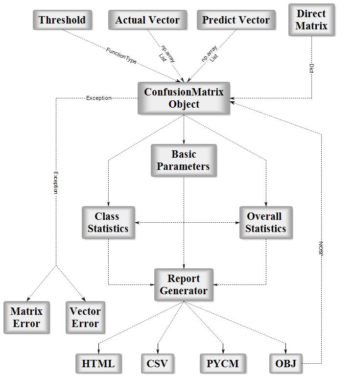
PyCM is a multi-class confusion matrix library written in Python that supports both input data vectors and direct matrix, and a proper tool for post-classification model evaluation that supports most classes and overall statistics parameters. PyCM is the swiss-army knife of confusion matrices, targeted mainly at data scientists that need a broad array of metrics for predictive models and an accurate evaluation of large variety of classifiers.
Installation
Source Code
- Download Version 1.0 or Latest Source
- Run
pip install -r requirements.txtorpip3 install -r requirements.txt(Need root access) - Run
python3 setup.py installorpython setup.py install(Need root access)
PyPI
- Check Python Packaging User Guide
- Run
pip install pycm --upgradeorpip3 install pycm --upgrade(Need root access)
Easy Install
- Run
easy_install --upgrade pycm(Need root access)
Usage
From Vector
from pycm import *
y_actu = [2, 0, 2, 2, 0, 1, 1, 2, 2, 0, 1, 2]
y_pred = [0, 0, 2, 1, 0, 2, 1, 0, 2, 0, 2, 2]
cm = ConfusionMatrix(y_actu, y_pred,digit=5)
- Notice : digit (the number of digits to the right of the decimal point in a number) is new in version 0.6 (default valaue : 5)
- Only for print and save
cm
pycm.ConfusionMatrix(classes: [0, 1, 2])
cm.actual_vector
[2, 0, 2, 2, 0, 1, 1, 2, 2, 0, 1, 2]
cm.predict_vector
[0, 0, 2, 1, 0, 2, 1, 0, 2, 0, 2, 2]
cm.classes
[0, 1, 2]
cm.class_stat
{'ACC': {0: 0.8333333333333334, 1: 0.75, 2: 0.5833333333333334},
 'BM': {0: 0.7777777777777777, 1: 0.2222222222222221, 2: 0.16666666666666652},
 'DOR': {0: 'None', 1: 3.999999999999998, 2: 1.9999999999999998},
 'ERR': {0: 0.16666666666666663, 1: 0.25, 2: 0.41666666666666663},
 'F0.5': {0: 0.6521739130434783,
  1: 0.45454545454545453,
  2: 0.5769230769230769},
 'F1': {0: 0.75, 1: 0.4, 2: 0.5454545454545454},
 'F2': {0: 0.8823529411764706, 1: 0.35714285714285715, 2: 0.5172413793103449},
 'FDR': {0: 0.4, 1: 0.5, 2: 0.4},
 'FN': {0: 0, 1: 2, 2: 3},
 'FNR': {0: 0.0, 1: 0.6666666666666667, 2: 0.5},
 'FOR': {0: 0.0, 1: 0.19999999999999996, 2: 0.4285714285714286},
 'FP': {0: 2, 1: 1, 2: 2},
 'FPR': {0: 0.2222222222222222,
  1: 0.11111111111111116,
  2: 0.33333333333333337},
 'G': {0: 0.7745966692414834, 1: 0.408248290463863, 2: 0.5477225575051661},
 'J': {0: 0.6, 1: 0.25, 2: 0.375},
 'LR+': {0: 4.5, 1: 2.9999999999999987, 2: 1.4999999999999998},
 'LR-': {0: 0.0, 1: 0.7500000000000001, 2: 0.75},
 'MCC': {0: 0.6831300510639732, 1: 0.25819888974716115, 2: 0.1690308509457033},
 'MK': {0: 0.6000000000000001, 1: 0.30000000000000004, 2: 0.17142857142857126},
 'N': {0: 9, 1: 9, 2: 6},
 'NPV': {0: 1.0, 1: 0.8, 2: 0.5714285714285714},
 'P': {0: 3, 1: 3, 2: 6},
 'POP': {0: 12, 1: 12, 2: 12},
 'PPV': {0: 0.6, 1: 0.5, 2: 0.6},
 'PRE': {0: 0.25, 1: 0.25, 2: 0.5},
 'RACC': {0: 0.10416666666666667,
  1: 0.041666666666666664,
  2: 0.20833333333333334},
 'RACCU': {0: 0.1111111111111111,
  1: 0.04340277777777778,
  2: 0.21006944444444442},
 'TN': {0: 7, 1: 8, 2: 4},
 'TNR': {0: 0.7777777777777778, 1: 0.8888888888888888, 2: 0.6666666666666666},
 'TON': {0: 7, 1: 10, 2: 7},
 'TOP': {0: 5, 1: 2, 2: 5},
 'TP': {0: 3, 1: 1, 2: 3},
 'TPR': {0: 1.0, 1: 0.3333333333333333, 2: 0.5}}
- Notice : cm.statistic_result in prev versions (<0.2)
cm.overall_stat
{'95% CI': (0.30438856248221097, 0.8622781041844558),
 'Bennett_S': 0.37500000000000006,
 'Chi-Squared': 6.6,
 'Chi-Squared DF': 4,
 'Conditional Entropy': 0.9591479170272448,
 'Cramer_V': 0.5244044240850757,
 'Cross Entropy': 1.5935164295556343,
 'Gwet_AC1': 0.3893129770992367,
 'Hamming Loss': 0.41666666666666663,
 'Joint Entropy': 2.4591479170272446,
 'KL Divergence': 0.09351642955563438,
 'Kappa': 0.35483870967741943,
 'Kappa 95% CI': (-0.07707577422109269, 0.7867531935759315),
 'Kappa No Prevalence': 0.16666666666666674,
 'Kappa Standard Error': 0.2203645326012817,
 'Kappa Unbiased': 0.34426229508196726,
 'Lambda A': 0.16666666666666666,
 'Lambda B': 0.42857142857142855,
 'Mutual Information': 0.5242078379544426,
 'Overall_ACC': 0.5833333333333334,
 'Overall_J': (1.225, 0.4083333333333334),
 'Overall_RACC': 0.3541666666666667,
 'Overall_RACCU': 0.3645833333333333,
 'PPV_Macro': 0.5666666666666668,
 'PPV_Micro': 0.5833333333333334,
 'Phi-Squared': 0.5499999999999999,
 'Reference Entropy': 1.5,
 'Response Entropy': 1.4833557549816874,
 'Scott_PI': 0.34426229508196726,
 'Standard Error': 0.14231876063832777,
 'Strength_Of_Agreement(Altman)': 'Fair',
 'Strength_Of_Agreement(Cicchetti)': 'Poor',
 'Strength_Of_Agreement(Fleiss)': 'Poor',
 'Strength_Of_Agreement(Landis and Koch)': 'Fair',
 'TPR_Macro': 0.611111111111111,
 'TPR_Micro': 0.5833333333333334}
- Notice : new in version 0.3
cm.table
{0: {0: 3, 1: 0, 2: 0}, 1: {0: 0, 1: 1, 2: 2}, 2: {0: 2, 1: 1, 2: 3}}
import numpy
y_actu = numpy.array([2, 0, 2, 2, 0, 1, 1, 2, 2, 0, 1, 2])
y_pred = numpy.array([0, 0, 2, 1, 0, 2, 1, 0, 2, 0, 2, 2])
cm = ConfusionMatrix(y_actu, y_pred,digit=5)
cm
pycm.ConfusionMatrix(classes: [0, 1, 2])
- Notice : numpy.array support in version>0.7
Direct CM
cm2 = ConfusionMatrix(matrix={0: {0: 3, 1: 0, 2: 0}, 1: {0: 0, 1: 1, 2: 2}, 2: {0: 2, 1: 1, 2: 3}},digit=5)
cm2
pycm.ConfusionMatrix(classes: [0, 1, 2])
cm2.actual_vector
cm2.predict_vector
cm2.classes
[0, 1, 2]
cm2.class_stat
{'ACC': {0: 0.8333333333333334, 1: 0.75, 2: 0.5833333333333334},
 'BM': {0: 0.7777777777777777, 1: 0.2222222222222221, 2: 0.16666666666666652},
 'DOR': {0: 'None', 1: 3.999999999999998, 2: 1.9999999999999998},
 'ERR': {0: 0.16666666666666663, 1: 0.25, 2: 0.41666666666666663},
 'F0.5': {0: 0.6521739130434783,
  1: 0.45454545454545453,
  2: 0.5769230769230769},
 'F1': {0: 0.75, 1: 0.4, 2: 0.5454545454545454},
 'F2': {0: 0.8823529411764706, 1: 0.35714285714285715, 2: 0.5172413793103449},
 'FDR': {0: 0.4, 1: 0.5, 2: 0.4},
 'FN': {0: 0, 1: 2, 2: 3},
 'FNR': {0: 0.0, 1: 0.6666666666666667, 2: 0.5},
 'FOR': {0: 0.0, 1: 0.19999999999999996, 2: 0.4285714285714286},
 'FP': {0: 2, 1: 1, 2: 2},
 'FPR': {0: 0.2222222222222222,
  1: 0.11111111111111116,
  2: 0.33333333333333337},
 'G': {0: 0.7745966692414834, 1: 0.408248290463863, 2: 0.5477225575051661},
 'J': {0: 0.6, 1: 0.25, 2: 0.375},
 'LR+': {0: 4.5, 1: 2.9999999999999987, 2: 1.4999999999999998},
 'LR-': {0: 0.0, 1: 0.7500000000000001, 2: 0.75},
 'MCC': {0: 0.6831300510639732, 1: 0.25819888974716115, 2: 0.1690308509457033},
 'MK': {0: 0.6000000000000001, 1: 0.30000000000000004, 2: 0.17142857142857126},
 'N': {0: 9, 1: 9, 2: 6},
 'NPV': {0: 1.0, 1: 0.8, 2: 0.5714285714285714},
 'P': {0: 3, 1: 3, 2: 6},
 'POP': {0: 12, 1: 12, 2: 12},
 'PPV': {0: 0.6, 1: 0.5, 2: 0.6},
 'PRE': {0: 0.25, 1: 0.25, 2: 0.5},
 'RACC': {0: 0.10416666666666667,
  1: 0.041666666666666664,
  2: 0.20833333333333334},
 'RACCU': {0: 0.1111111111111111,
  1: 0.04340277777777778,
  2: 0.21006944444444442},
 'TN': {0: 7, 1: 8, 2: 4},
 'TNR': {0: 0.7777777777777778, 1: 0.8888888888888888, 2: 0.6666666666666666},
 'TON': {0: 7, 1: 10, 2: 7},
 'TOP': {0: 5, 1: 2, 2: 5},
 'TP': {0: 3, 1: 1, 2: 3},
 'TPR': {0: 1.0, 1: 0.3333333333333333, 2: 0.5}}
cm.overall_stat
{'95% CI': (0.30438856248221097, 0.8622781041844558),
 'Bennett_S': 0.37500000000000006,
 'Chi-Squared': 6.6,
 'Chi-Squared DF': 4,
 'Conditional Entropy': 0.9591479170272448,
 'Cramer_V': 0.5244044240850757,
 'Cross Entropy': 1.5935164295556343,
 'Gwet_AC1': 0.3893129770992367,
 'Hamming Loss': 0.41666666666666663,
 'Joint Entropy': 2.4591479170272446,
 'KL Divergence': 0.09351642955563438,
 'Kappa': 0.35483870967741943,
 'Kappa 95% CI': (-0.07707577422109269, 0.7867531935759315),
 'Kappa No Prevalence': 0.16666666666666674,
 'Kappa Standard Error': 0.2203645326012817,
 'Kappa Unbiased': 0.34426229508196726,
 'Lambda A': 0.16666666666666666,
 'Lambda B': 0.42857142857142855,
 'Mutual Information': 0.5242078379544426,
 'Overall_ACC': 0.5833333333333334,
 'Overall_J': (1.225, 0.4083333333333334),
 'Overall_RACC': 0.3541666666666667,
 'Overall_RACCU': 0.3645833333333333,
 'PPV_Macro': 0.5666666666666668,
 'PPV_Micro': 0.5833333333333334,
 'Phi-Squared': 0.5499999999999999,
 'Reference Entropy': 1.5,
 'Response Entropy': 1.4833557549816874,
 'Scott_PI': 0.34426229508196726,
 'Standard Error': 0.14231876063832777,
 'Strength_Of_Agreement(Altman)': 'Fair',
 'Strength_Of_Agreement(Cicchetti)': 'Poor',
 'Strength_Of_Agreement(Fleiss)': 'Poor',
 'Strength_Of_Agreement(Landis and Koch)': 'Fair',
 'TPR_Macro': 0.611111111111111,
 'TPR_Micro': 0.5833333333333334}
- Notice : new in version 0.8.1
- In direct matrix mode actual_vector and predict_vector are empty
Activation Threshold
threshold is added in Version 0.9 for real value prediction.
For more information visit Example3
- Notice : new in version 0.9
Load From File
file is added in Version 0.9.5 in order to load saved confusion matrix with .obj format generated by save_obj method.
For more information visit Example4
- Notice : new in version 0.9.5
Acceptable Data Types
actual_vector: pythonlistor numpyarrayof any stringable objectspredict_vector: pythonlistor numpyarrayof any stringable objectsmatrix:dictdigit:intthreshold:FunctionType (function or lambda)file:File object
- run
help(ConfusionMatrix)for more information
Basic Parameters
TP (True positive / hit)
A true positive test result is one that detects the condition when the condition is present. (correctly identified)
cm.TP
{0: 3, 1: 1, 2: 3}
TN (True negative/correct rejection)
A true negative test result is one that does not detect the condition when the condition is absent. (correctly rejected)
cm.TN
{0: 7, 1: 8, 2: 4}
FP (False positive/false alarm/Type I error)
A false positive test result is one that detects the condition when the condition is absent. (incorrectly identified)
cm.FP
{0: 2, 1: 1, 2: 2}
FN (False negative/miss/Type II error)
A false negative test result is one that does not detect the condition when the condition is present. (incorrectly rejected)
cm.FN
{0: 0, 1: 2, 2: 3}
P (Condition positive)
(number of) positive samples
cm.P
{0: 3, 1: 3, 2: 6}
N (Condition negative)
(number of) negative samples
cm.N
{0: 9, 1: 9, 2: 6}
TOP (Test outcome positive)
(number of) positive outcomes
cm.TOP
{0: 5, 1: 2, 2: 5}
TON (Test outcome negative)
(number of) negative outcomes
cm.TON
{0: 7, 1: 10, 2: 7}
POP (Population)
cm.POP
{0: 12, 1: 12, 2: 12}
- For more information visit here
Class Statistics
TPR (sensitivity, recall, hit rate, or true positive rate)
Sensitivity (also called the true positive rate, the recall, or probability of detection in some fields) measures the proportion of positives that are correctly identified as such (e.g. the percentage of sick people who are correctly identified as having the condition).
For more information visit here
cm.TPR
{0: 1.0, 1: 0.3333333333333333, 2: 0.5}
TNR (specificity or true negative rate)
Specificity (also called the true negative rate) measures the proportion of negatives that are correctly identified as such (e.g. the percentage of healthy people who are correctly identified as not having the condition).
For more information visit here
cm.TNR
{0: 0.7777777777777778, 1: 0.8888888888888888, 2: 0.6666666666666666}
PPV (precision or positive predictive value)
Predictive value positive is the proportion of positives that correspond to the presence of the condition
For more information visit here
cm.PPV
{0: 0.6, 1: 0.5, 2: 0.6}
NPV (negative predictive value)
Predictive value negative is the proportion of negatives that correspond to the absence of the condition
For more information visit here
cm.NPV
{0: 1.0, 1: 0.8, 2: 0.5714285714285714}
FNR (miss rate or false negative rate)
The false negative rate is the proportion of positives which yield negative test outcomes with the test, i.e., the conditional probability of a negative test result given that the condition being looked for is present.
For more information visit here
cm.FNR
{0: 0.0, 1: 0.6666666666666667, 2: 0.5}
FPR (fall-out or false positive rate)
The false positive rate is the proportion of all negatives that still yield positive test outcomes, i.e., the conditional probability of a positive test result given an event that was not present.
The false positive rate is equal to the significance level. The specificity of the test is equal to 1 minus the false positive rate.
For more information visit here
cm.FPR
{0: 0.2222222222222222, 1: 0.11111111111111116, 2: 0.33333333333333337}
FDR (false discovery rate)
The false discovery rate (FDR) is a method of conceptualizing the rate of type I errors in null hypothesis testing when conducting multiple comparisons. FDR-controlling procedures are designed to control the expected proportion of "discoveries" (rejected null hypotheses) that are false (incorrect rejections)
For more information visit here
cm.FDR
{0: 0.4, 1: 0.5, 2: 0.4}
FOR (false omission rate)
False omission rate (FOR) is a statistical method used in multiple hypothesis testing to correct for multiple comparisons and it is the complement of the negative predictive value. It measures the proportion of false negatives which are incorrectly rejected.
For more information visit here
cm.FOR
{0: 0.0, 1: 0.19999999999999996, 2: 0.4285714285714286}
ACC (accuracy)
The accuracy is the number of correct predictions from all predictions made
For more information visit here
cm.ACC
{0: 0.8333333333333334, 1: 0.75, 2: 0.5833333333333334}
ERR(Error rate)
The accuracy is the number of incorrect predictions from all predictions made
cm.ERR
{0: 0.16666666666666663, 1: 0.25, 2: 0.41666666666666663}
- Notice : new in version 0.4
FBeta-Score
In statistical analysis of classification, the F1 score (also F-score or F-measure) is a measure of a test's accuracy. It considers both the precision p and the recall r of the test to compute the score. The F1 score is the harmonic average of the precision and recall, where an F1 score reaches its best value at 1 (perfect precision and recall) and worst at 0.
For more information visit here
cm.F1
{0: 0.75, 1: 0.4, 2: 0.5454545454545454}
cm.F05
{0: 0.6521739130434783, 1: 0.45454545454545453, 2: 0.5769230769230769}
cm.F2
{0: 0.8823529411764706, 1: 0.35714285714285715, 2: 0.5172413793103449}
cm.F_beta(Beta=4)
{0: 0.9622641509433962, 1: 0.34, 2: 0.504950495049505}
- Notice : new in version 0.4
MCC (Matthews correlation coefficient)
The Matthews correlation coefficient is used in machine learning as a measure of the quality of binary (two-class) classifications, introduced by biochemist Brian W. Matthews in 1975. It takes into account true and false positives and negatives and is generally regarded as a balanced measure which can be used even if the classes are of very different sizes.The MCC is in essence a correlation coefficient between the observed and predicted binary classifications; it returns a value between −1 and +1. A coefficient of +1 represents a perfect prediction, 0 no better than random prediction and −1 indicates total disagreement between prediction and observation.
For more information visit here
cm.MCC
{0: 0.6831300510639732, 1: 0.25819888974716115, 2: 0.1690308509457033}
BM (Informedness or Bookmaker Informedness)
The informedness of a prediction method as captured by a contingency matrix is defined as the probability that the prediction method will make a correct decision as opposed to guessing and is calculated using the bookmaker algorithm.
cm.BM
{0: 0.7777777777777777, 1: 0.2222222222222221, 2: 0.16666666666666652}
MK (Markedness)
In statistics and psychology, the social science concept of markedness is quantified as a measure of how much one variable is marked as a predictor or possible cause of another, and is also known as Δp (deltaP) in simple two-choice cases
cm.MK
{0: 0.6000000000000001, 1: 0.30000000000000004, 2: 0.17142857142857126}
PLR (Positive likelihood ratio)
Likelihood ratios are used for assessing the value of performing a diagnostic test. They use the sensitivity and specificity of the test to determine whether a test result usefully changes the probability that a condition (such as a disease state) exists. The first description of the use of likelihood ratios for decision rules was made at a symposium on information theory in 1954.
For more information visit here
cm.PLR
{0: 4.5, 1: 2.9999999999999987, 2: 1.4999999999999998}
NLR (Negative likelihood ratio)
Likelihood ratios are used for assessing the value of performing a diagnostic test. They use the sensitivity and specificity of the test to determine whether a test result usefully changes the probability that a condition (such as a disease state) exists. The first description of the use of likelihood ratios for decision rules was made at a symposium on information theory in 1954.
For more information visit here
cm.NLR
{0: 0.0, 1: 0.7500000000000001, 2: 0.75}
DOR (Diagnostic odds ratio)
The diagnostic odds ratio is a measure of the effectiveness of a diagnostic test. It is defined as the ratio of the odds of the test being positive if the subject has a disease relative to the odds of the test being positive if the subject does not have the disease.
For more information visit here
cm.DOR
{0: 'None', 1: 3.999999999999998, 2: 1.9999999999999998}
PRE (Prevalence)
Prevalence is a statistical concept referring to the number of cases of a disease that are present in a particular population at a given time (Reference Likelihood)
For more information visit here
cm.PRE
{0: 0.25, 1: 0.25, 2: 0.5}
G (G-measure geometric mean of precision and sensitivity)
Geometric mean of precision and sensitivity
For more information visit here
cm.G
{0: 0.7745966692414834, 1: 0.408248290463863, 2: 0.5477225575051661}
RACC(Random accuracy)
The expected accuracy from a strategy of randomly guessing categories according to reference and response distributions
cm.RACC
{0: 0.10416666666666667, 1: 0.041666666666666664, 2: 0.20833333333333334}
- Notice : new in version 0.3
RACCU(Random accuracy unbiased)
The expected accuracy from a strategy of randomly guessing categories according to the average of the reference and response distributions
cm.RACCU
{0: 0.1111111111111111, 1: 0.04340277777777778, 2: 0.21006944444444442}
- Notice : new in version 0.8.1
J (Jaccard index)
The Jaccard index, also known as Intersection over Union and the Jaccard similarity coefficient (originally coined coefficient de communauté by Paul Jaccard), is a statistic used for comparing the similarity and diversity of sample sets.
For more information visit here
cm.J
{0: 0.6, 1: 0.25, 2: 0.375}
- Notice : new in version 0.9
Overall Statistics
Kappa (Nominal)
Kappa is a statistic which measures inter-rater agreement for qualitative (categorical) items. It is generally thought to be a more robust measure than simple percent agreement calculation, as kappa takes into account the possibility of the agreement occurring by chance.
For more information visit here
cm.Kappa
0.35483870967741943
- Notice : new in version 0.3
Kappa Unbiased
The unbiased kappa value is defined in terms of total accuracy and a slightly different computation of expected likelihood that averages the reference and response probabilities
cm.KappaUnbiased
0.34426229508196726
- Notice : new in version 0.8.1
Kappa No Prevalence
The kappa statistic adjusted for prevalence
cm.KappaNoPrevalence
0.16666666666666674
- Notice : new in version 0.8.1
Kappa 95% CI
Kappa 95% Confidence Interval
cm.Kappa_SE
0.2203645326012817
cm.Kappa_CI
(-0.07707577422109269, 0.7867531935759315)
- Notice : new in version 0.7
Chi-Squared
Pearson's chi-squared test is a statistical test applied to sets of categorical data to evaluate how likely it is that any observed difference between the sets arose by chance. It is suitable for unpaired data from large samples.
For more information visit here
cm.Chi_Squared
6.6
- Notice : new in version 0.7
Chi-Squared DF
Number of degrees of freedom of this confusion matrix for the chi-squared statistic
cm.DF
4
- Notice : new in version 0.7
Phi-Squared
In statistics, the phi coefficient (or mean square contingency coefficient) is a measure of association for two binary variables. Introduced by Karl Pearson, this measure is similar to the Pearson correlation coefficient in its interpretation. In fact, a Pearson correlation coefficient estimated for two binary variables will return the phi coefficient
For more information visit here
cm.Phi_Squared
0.5499999999999999
- Notice : new in version 0.7
Cramer's V
In statistics, Cramér's V (sometimes referred to as Cramér's phi) is a measure of association between two nominal variables, giving a value between 0 and +1 (inclusive). It is based on Pearson's chi-squared statistic and was published by Harald Cramér in 1946.
For more information visit here
cm.V
0.5244044240850757
- Notice : new in version 0.7
95% CI
In statistics, a confidence interval (CI) is a type of interval estimate (of a population parameter) that is computed from the observed data. The confidence level is the frequency (i.e., the proportion) of possible confidence intervals that contain the true value of their corresponding parameter. In other words, if confidence intervals are constructed using a given confidence level in an infinite number of independent experiments, the proportion of those intervals that contain the true value of the parameter will match the confidence level.
For more information visit here
cm.CI
(0.30438856248221097, 0.8622781041844558)
cm.SE
0.14231876063832777
- Notice : new in version 0.7
Bennett et al.'s S score (Nominal)
Bennett, Alpert & Goldstein’s S is a statistical measure of inter-rater agreement. It was created by Bennett et al. in 1954 Bennett et al. suggested adjusting inter-rater reliability to accommodate the percentage of rater agreement that might be expected by chance was a better measure than simple agreement between raters.
For more information visit here
cm.S
0.37500000000000006
- Notice : new in version 0.5
Scott's pi (Nominal)
Scott's pi (named after William A. Scott) is a statistic for measuring inter-rater reliability for nominal data in communication studies. Textual entities are annotated with categories by different annotators, and various measures are used to assess the extent of agreement between the annotators, one of which is Scott's pi. Since automatically annotating text is a popular problem in natural language processing, and goal is to get the computer program that is being developed to agree with the humans in the annotations it creates, assessing the extent to which humans agree with each other is important for establishing a reasonable upper limit on computer performance.
For more information visit here
cm.PI
0.34426229508196726
- Notice : new in version 0.5
Gwet's AC1
AC1 was originally introduced by Gwet in 2001 (Gwet, 2001). The interpretation of AC1 is similar to generalized kappa (Fleiss, 1971), which is used to assess interrater reliability of when there are multiple raters. Gwet (2002) demonstrated that AC1 can overcome the limitations that kappa is sensitive to trait prevalence and rater's classification probabilities (i.e., marginal probabilities), whereas AC1 provides more robust measure of interrater reliability
cm.AC1
0.3893129770992367
- Notice : new in version 0.5
Reference Entropy
The entropy of the decision problem itself as defined by the counts for the reference. The entropy of a distribution is the average negative log probability of outcomes
cm.ReferenceEntropy
1.5
- Notice : new in version 0.8.1
Response Entropy
The entropy of the response distribution. The entropy of a distribution is the average negative log probability of outcomes
cm.ResponseEntropy
1.4833557549816874
- Notice : new in version 0.8.1
Cross Entropy
The cross-entropy of the response distribution against the reference distribution. The cross-entropy is defined by the negative log probabilities of the response distribution weighted by the reference distribution
cm.CrossEntropy
1.5935164295556343
- Notice : new in version 0.8.1
Joint Entropy
The entropy of the joint reference and response distribution as defined by the underlying matrix
cm.JointEntropy
2.4591479170272446
- Notice : new in version 0.8.1
Conditional Entropy
The entropy of the distribution of categories in the response given that the reference category was as specified
cm.ConditionalEntropy
0.9591479170272448
- Notice : new in version 0.8.1
Kullback-Liebler (KL) divergence
In mathematical statistics, the Kullback–Leibler divergence (also called relative entropy) is a measure of how one probability distribution diverges from a second, expected probability distribution
For more information visit here
cm.KL
0.09351642955563438
- Notice : new in version 0.8.1
Mutual Information
Mutual information is defined Kullback-Lieblier divergence, between the product of the individual distributions and the joint distribution. Mutual information is symmetric. We could also subtract the conditional entropy of the reference given the response from the reference entropy to get the same result.
cm.MutualInformation
0.5242078379544426
- Notice : new in version 0.8.1
Goodman and Kruskal's lambda A
In probability theory and statistics, Goodman & Kruskal's lambda is a measure of proportional reduction in error in cross tabulation analysis.
For more information visit here
cm.LambdaA
0.16666666666666666
- Notice : new in version 0.8.1
Goodman and Kruskal's lambda B
In probability theory and statistics, Goodman & Kruskal's lambda is a measure of proportional reduction in error in cross tabulation analysis
For more information visit here
cm.LambdaB
0.42857142857142855
- Notice : new in version 0.8.1
SOA1 (Strength of Agreement, Landis and Koch benchmark)
| Kappa | Strength of Agreement |
| 0 > | Poor |
| 0 - 0.20 | Slight |
| 0.21 – 0.40 | Fair |
| 0.41 – 0.60 | Moderate |
| 0.61 – 0.80 | Substantial |
| 0.81 – 1.00 | Almost perfect |
cm.SOA1
'Fair'
- Notice : new in version 0.3
SOA2 (Strength of Agreement, : Fleiss’ benchmark)
| Kappa | Strength of Agreement |
| 0.40 > | Poor |
| 0.4 - 0.75 | Intermediate to Good |
| More than 0.75 | Excellent |
cm.SOA2
'Poor'
- Notice : new in version 0.4
SOA3 (Strength of Agreement, Altman’s benchmark)
| Kappa | Strength of Agreement |
| 0.2 > | Poor |
| 0.21 – 0.40 | Fair |
| 0.41 – 0.60 | Moderate |
| 0.61 – 0.80 | Good |
| 0.81 – 1.00 | Very Good |
cm.SOA3
'Fair'
- Notice : new in version 0.4
SOA4 (Strength of Agreement, Cicchetti’s benchmark)
| Kappa | Strength of Agreement |
| 0.4 > | Poor |
| 0.4 – 0.59 | Fair |
| 0.6 – 0.74 | Good |
| 0.74 – 1.00 | Excellent |
cm.SOA4
'Poor'
- Notice : new in version 0.7
Overall_ACC
cm.Overall_ACC
0.5833333333333334
- Notice : new in version 0.4
Overall_RACC
cm.Overall_RACC
0.3541666666666667
- Notice : new in version 0.4
Overall_RACCU
cm.Overall_RACCU
0.3645833333333333
- Notice : new in version 0.8.1
PPV_Micro
cm.PPV_Micro
0.5833333333333334
- Notice : new in version 0.4
TPR_Micro
cm.TPR_Micro
0.5833333333333334
- Notice : new in version 0.4
PPV_Macro
cm.PPV_Macro
0.5666666666666668
- Notice : new in version 0.4
TPR_Macro
cm.TPR_Macro
0.611111111111111
- Notice : new in version 0.4
Overall_J
cm.Overall_J
(1.225, 0.4083333333333334)
- Notice : new in version 0.9
Hamming Loss
The hamming_loss computes the average Hamming loss or Hamming distance between two sets of samples
cm.HammingLoss
0.41666666666666663
- Notice : new in version 1.0
Print
Full
print(cm)
Predict          0        1        2
Actual
0                3        0        0
1                0        1        2
2                2        1        3


Overall Statistics :

95% CI                                                           (0.30439,0.86228)
Bennett_S                                                        0.375
Chi-Squared                                                      6.6
Chi-Squared DF                                                   4
Conditional Entropy                                              0.95915
Cramer_V                                                         0.5244
Cross Entropy                                                    1.59352
Gwet_AC1                                                         0.38931
Hamming Loss                                                     0.41667
Joint Entropy                                                    2.45915
KL Divergence                                                    0.09352
Kappa                                                            0.35484
Kappa 95% CI                                                     (-0.07708,0.78675)
Kappa No Prevalence                                              0.16667
Kappa Standard Error                                             0.22036
Kappa Unbiased                                                   0.34426
Lambda A                                                         0.16667
Lambda B                                                         0.42857
Mutual Information                                               0.52421
Overall_ACC                                                      0.58333
Overall_J                                                        (1.225,0.40833)
Overall_RACC                                                     0.35417
Overall_RACCU                                                    0.36458
PPV_Macro                                                        0.56667
PPV_Micro                                                        0.58333
Phi-Squared                                                      0.55
Reference Entropy                                                1.5
Response Entropy                                                 1.48336
Scott_PI                                                         0.34426
Standard Error                                                   0.14232
Strength_Of_Agreement(Altman)                                    Fair
Strength_Of_Agreement(Cicchetti)                                 Poor
Strength_Of_Agreement(Fleiss)                                    Poor
Strength_Of_Agreement(Landis and Koch)                           Fair
TPR_Macro                                                        0.61111
TPR_Micro                                                        0.58333

Class Statistics :

Classes                                                          0                       1                       2
ACC(Accuracy)                                                    0.83333                 0.75                    0.58333
BM(Informedness or bookmaker informedness)                       0.77778                 0.22222                 0.16667
DOR(Diagnostic odds ratio)                                       None                    4.0                     2.0
ERR(Error rate)                                                  0.16667                 0.25                    0.41667
F0.5(F0.5 score)                                                 0.65217                 0.45455                 0.57692
F1(F1 score - harmonic mean of precision and sensitivity)        0.75                    0.4                     0.54545
F2(F2 score)                                                     0.88235                 0.35714                 0.51724
FDR(False discovery rate)                                        0.4                     0.5                     0.4
FN(False negative/miss/type 2 error)                             0                       2                       3
FNR(Miss rate or false negative rate)                            0.0                     0.66667                 0.5
FOR(False omission rate)                                         0.0                     0.2                     0.42857
FP(False positive/type 1 error/false alarm)                      2                       1                       2
FPR(Fall-out or false positive rate)                             0.22222                 0.11111                 0.33333
G(G-measure geometric mean of precision and sensitivity)         0.7746                  0.40825                 0.54772
J(Jaccard index)                                                 0.6                     0.25                    0.375
LR+(Positive likelihood ratio)                                   4.5                     3.0                     1.5
LR-(Negative likelihood ratio)                                   0.0                     0.75                    0.75
MCC(Matthews correlation coefficient)                            0.68313                 0.2582                  0.16903
MK(Markedness)                                                   0.6                     0.3                     0.17143
N(Condition negative)                                            9                       9                       6
NPV(Negative predictive value)                                   1.0                     0.8                     0.57143
P(Condition positive)                                            3                       3                       6
POP(Population)                                                  12                      12                      12
PPV(Precision or positive predictive value)                      0.6                     0.5                     0.6
PRE(Prevalence)                                                  0.25                    0.25                    0.5
RACC(Random accuracy)                                            0.10417                 0.04167                 0.20833
RACCU(Random accuracy unbiased)                                  0.11111                 0.0434                  0.21007
TN(True negative/correct rejection)                              7                       8                       4
TNR(Specificity or true negative rate)                           0.77778                 0.88889                 0.66667
TON(Test outcome negative)                                       7                       10                      7
TOP(Test outcome positive)                                       5                       2                       5
TP(True positive/hit)                                            3                       1                       3
TPR(Sensitivity, recall, hit rate, or true positive rate)        1.0                     0.33333                 0.5
Matrix
cm.matrix()
Predict          0        1        2
Actual
0                3        0        0
1                0        1        2
2                2        1        3
Normalized Matrix
cm.normalized_matrix()
Predict          0              1              2
Actual
0                1.0            0.0            0.0
1                0.0            0.33333        0.66667
2                0.33333        0.16667        0.5
Stat
cm.stat()
Overall Statistics :

95% CI                                                           (0.30439,0.86228)
Bennett_S                                                        0.375
Chi-Squared                                                      6.6
Chi-Squared DF                                                   4
Conditional Entropy                                              0.95915
Cramer_V                                                         0.5244
Cross Entropy                                                    1.59352
Gwet_AC1                                                         0.38931
Hamming Loss                                                     0.41667
Joint Entropy                                                    2.45915
KL Divergence                                                    0.09352
Kappa                                                            0.35484
Kappa 95% CI                                                     (-0.07708,0.78675)
Kappa No Prevalence                                              0.16667
Kappa Standard Error                                             0.22036
Kappa Unbiased                                                   0.34426
Lambda A                                                         0.16667
Lambda B                                                         0.42857
Mutual Information                                               0.52421
Overall_ACC                                                      0.58333
Overall_J                                                        (1.225,0.40833)
Overall_RACC                                                     0.35417
Overall_RACCU                                                    0.36458
PPV_Macro                                                        0.56667
PPV_Micro                                                        0.58333
Phi-Squared                                                      0.55
Reference Entropy                                                1.5
Response Entropy                                                 1.48336
Scott_PI                                                         0.34426
Standard Error                                                   0.14232
Strength_Of_Agreement(Altman)                                    Fair
Strength_Of_Agreement(Cicchetti)                                 Poor
Strength_Of_Agreement(Fleiss)                                    Poor
Strength_Of_Agreement(Landis and Koch)                           Fair
TPR_Macro                                                        0.61111
TPR_Micro                                                        0.58333

Class Statistics :

Classes                                                          0                       1                       2
ACC(Accuracy)                                                    0.83333                 0.75                    0.58333
BM(Informedness or bookmaker informedness)                       0.77778                 0.22222                 0.16667
DOR(Diagnostic odds ratio)                                       None                    4.0                     2.0
ERR(Error rate)                                                  0.16667                 0.25                    0.41667
F0.5(F0.5 score)                                                 0.65217                 0.45455                 0.57692
F1(F1 score - harmonic mean of precision and sensitivity)        0.75                    0.4                     0.54545
F2(F2 score)                                                     0.88235                 0.35714                 0.51724
FDR(False discovery rate)                                        0.4                     0.5                     0.4
FN(False negative/miss/type 2 error)                             0                       2                       3
FNR(Miss rate or false negative rate)                            0.0                     0.66667                 0.5
FOR(False omission rate)                                         0.0                     0.2                     0.42857
FP(False positive/type 1 error/false alarm)                      2                       1                       2
FPR(Fall-out or false positive rate)                             0.22222                 0.11111                 0.33333
G(G-measure geometric mean of precision and sensitivity)         0.7746                  0.40825                 0.54772
J(Jaccard index)                                                 0.6                     0.25                    0.375
LR+(Positive likelihood ratio)                                   4.5                     3.0                     1.5
LR-(Negative likelihood ratio)                                   0.0                     0.75                    0.75
MCC(Matthews correlation coefficient)                            0.68313                 0.2582                  0.16903
MK(Markedness)                                                   0.6                     0.3                     0.17143
N(Condition negative)                                            9                       9                       6
NPV(Negative predictive value)                                   1.0                     0.8                     0.57143
P(Condition positive)                                            3                       3                       6
POP(Population)                                                  12                      12                      12
PPV(Precision or positive predictive value)                      0.6                     0.5                     0.6
PRE(Prevalence)                                                  0.25                    0.25                    0.5
RACC(Random accuracy)                                            0.10417                 0.04167                 0.20833
RACCU(Random accuracy unbiased)                                  0.11111                 0.0434                  0.21007
TN(True negative/correct rejection)                              7                       8                       4
TNR(Specificity or true negative rate)                           0.77778                 0.88889                 0.66667
TON(Test outcome negative)                                       7                       10                      7
TOP(Test outcome positive)                                       5                       2                       5
TP(True positive/hit)                                            3                       1                       3
TPR(Sensitivity, recall, hit rate, or true positive rate)        1.0                     0.33333                 0.5
- Notice : cm.params() in prev versions (<0.2)
Save
.pycm file
cm.save_stat("cm1")
{'Message': 'D:\\For Asus Laptop\\projects\\pycm\\Document\\cm1.pycm',
 'Status': True}
cm.save_stat("cm1asdasd/")
{'Message': "[Errno 2] No such file or directory: 'cm1asdasd/.pycm'",
 'Status': False}
- Notice : new in version 0.4
HTML
cm.save_html("cm1")
{'Message': 'D:\\For Asus Laptop\\projects\\pycm\\Document\\cm1.html',
 'Status': True}
cm.save_html("cm1asdasd/")
{'Message': "[Errno 2] No such file or directory: 'cm1asdasd/.html'",
 'Status': False}
- Notice : new in version 0.5
CSV
cm.save_csv("cm1")
{'Message': 'D:\\For Asus Laptop\\projects\\pycm\\Document\\cm1.csv',
 'Status': True}
cm.save_csv("cm1asdasd/")
{'Message': "[Errno 2] No such file or directory: 'cm1asdasd/.csv'",
 'Status': False}
- Notice : new in version 0.6
OBJ
cm.save_obj("cm1")
{'Message': 'D:\\For Asus Laptop\\projects\\pycm\\Document\\cm1.obj',
 'Status': True}
cm.save_obj("cm1asdasd/")
{'Message': "[Errno 2] No such file or directory: 'cm1asdasd/.obj'",
 'Status': False}
- Notice : new in version 0.9.5
Input Errors
try:
    cm2=ConfusionMatrix(y_actu, 2)
except pycmVectorError as e:
    print(str(e))
Input Vectors Must Be List
try:
    cm3=ConfusionMatrix(y_actu, [1,2,3])
except pycmVectorError as e:
    print(str(e))
Input Vectors Must Be The Same Length
try:
    cm_4 = ConfusionMatrix([], [])
except pycmVectorError as e:
    print(str(e))
Input Vectors Are Empty
try:
    cm_5 = ConfusionMatrix([1,1,1,], [1,1,1,1])
except pycmVectorError as e:
    print(str(e))
Input Vectors Must Be The Same Length
try:
    cm3=ConfusionMatrix(matrix={})
except pycmMatrixError as e:
    print(str(e))
Input Confusion Matrix Format Error
try:
    cm_4=ConfusionMatrix(matrix={1:{1:2,"1":2},"1":{1:2,"1":3}})
except pycmMatrixError as e:
    print(str(e))
Input Matrix Classes Must Be Same Type
try:
    cm_5=ConfusionMatrix(matrix={1:{1:2}})
except pycmVectorError as e:
    print(str(e))
Number Of Classes < 2
- Notice : updated in version 0.8
Examples
References
1- J. R. Landis, G. G. Koch, “The measurement of observer agreement for categorical data. Biometrics,” in International Biometric Society, pp. 159–174, 1977.
2- D. M. W. Powers, “Evaluation: from precision, recall and f-measure to roc, informedness, markedness & correlation,” in Journal of Machine Learning Technologies, pp.37-63, 2011.
3- C. Sammut, G. Webb, “Encyclopedia of Machine Learning” in Springer, 2011.
4- J. L. Fleiss, “Measuring nominal scale agreement among many raters,” in Psychological Bulletin, pp. 378-382.
5- D.G. Altman, “Practical Statistics for Medical Research,” in Chapman and Hall, 1990.
6- K. L. Gwet, “Computing inter-rater reliability and its variance in the presence of high agreement,” in The British Journal of Mathematical and Statistical Psychology, pp. 29–48, 2008.”
7- W. A. Scott, “Reliability of content analysis: The case of nominal scaling,” in Public Opinion Quarterly, pp. 321–325, 1955.
8- E. M. Bennett, R. Alpert, and A. C. Goldstein, “Communication through limited response questioning,” in The Public Opinion Quarterly, pp. 303–308, 1954.
9- D. V. Cicchetti, "Guidelines, criteria, and rules of thumb for evaluating normed and standardized assessment instruments in psychology," in Psychological Assessment, pp. 284–290, 1994.
10- R.B. Davies, "Algorithm AS155: The Distributions of a Linear Combination of χ2 Random Variables," in Journal of the Royal Statistical Society, pp. 323–333, 1980.
11- S. Kullback, R. A. Leibler "On information and sufficiency," in Annals of Mathematical Statistics, pp. 79–86, 1951.
12- L. A. Goodman, W. H. Kruskal, "Measures of Association for Cross Classifications, IV: Simplification of Asymptotic Variances," in Journal of the American Statistical Association, pp. 415–421, 1972.
13- L. A. Goodman, W. H. Kruskal, "Measures of Association for Cross Classifications III: Approximate Sampling Theory," in Journal of the American Statistical Association, pp. 310–364, 1963.
14- T. Byrt, J. Bishop and J. B. Carlin, “Bias, prevalence, and kappa,” in Journal of Clinical Epidemiology pp. 423-429, 1993.
15- M. Shepperd, D. Bowes, and T. Hall, “Researcher Bias: The Use of Machine Learning in Software Defect Prediction,” in IEEE Transactions on Software Engineering, pp. 603-616, 2014.
16- X. Deng, Q. Liu, Y. Deng, and S. Mahadevan, “An improved method to construct basic probability assignment based on the confusion matrix for classification problem, ” in Information Sciences, pp.250-261, 2016.