The Discrete Fourier Transform
This Jupyter notebook is part of a collection of notebooks in the bachelors module Signals and Systems, Comunications Engineering, Universität Rostock. Please direct questions and suggestions to Sascha.Spors@uni-rostock.de.
Fast Fourier Transform
The discrete Fourier transformation (DFT) can be implemented computationally very efficiently by the fast Fourier transform (FFT). Various algorithms have been developed for the FFT resulting in various levels of computational efficiency for a wide range of DFT lengths. The concept of the so called radix-2 Cooley–Tukey algorithm is introduced in the following as representative.
Radix-2 Decimation-in-Time Algorithm
Let's first consider the straightforward implementation of the DFT $X[\mu] = \text{DFT}_N \{ x[k] \}$ by its definition
\begin{equation} X[\mu] = \sum_{k=0}^{N-1} x[k] \, w_N^{\mu k} \end{equation}where $w_N = e^{-j \frac{2 \pi}{N}}$. Evaluation of the definition for $\mu = 0,1,\dots,N-1$ requires $N^2$ complex multiplications and $N \cdot (N-1)$ complex additions. The numerical complexity of the DFT scales consequently on the order of $\mathcal{O} (N^2)$.
The basic idea of the radix-2 decimation-in-time (DIT) algorithm is to decompose the computation of the DFT into two summations: one over the even indexes $k$ of the signal $x[k]$ and one over the odd indexes. Splitting the definition of the DFT for even lengths $N$ and rearranging terms yields
\begin{align} X[\mu] &= \sum_{\kappa = 0}^{\frac{N}{2} - 1} x[2 \kappa] \, w_N^{\mu 2 \kappa} + \sum_{\kappa = 0}^{\frac{N}{2} - 1} x[2 \kappa + 1] \, w_N^{\mu (2 \kappa + 1)} \\ &= \sum_{\kappa = 0}^{\frac{N}{2} - 1} x[2 \kappa] \, w_{\frac{N}{2}}^{\mu \kappa} + w_N^{\mu} \sum_{\kappa = 0}^{\frac{N}{2} - 1} \, x[2 \kappa + 1] w_{\frac{N}{2}}^{\mu \kappa} \\ &= X_1[\mu] + w_N^{\mu} \cdot X_2[\mu] \end{align}It follows from the last equality that the DFT can be decomposed into two DFTs $X_1[\mu]$ and $X_2[\mu]$ of length $\frac{N}{2}$ operating on the even and odd indexes of the signal $x[k]$. The decomposed DFT requires $2 \cdot (\frac{N}{2})^2 + N$ complex multiplications and $2 \cdot \frac{N}{2} \cdot (\frac{N}{2} -1) + N$ complex additions. For a length $N = 2^w$ with $w \in \mathbb{N}$ which is a power of two this principle can be applied recursively till a DFT of length $2$ is reached. This comprises then the radix-2 DIT algorithm. It requires $\frac{N}{2} \log_2 N$ complex multiplications and $N \log_2 N$ complex additions. The numerical complexity of the FFT algorithm scales consequently on the order of $\mathcal{O} (N \log_2 N)$. The notation DIT is due to the fact that the decomposition is performed with respect to the (time-domain) signal $x[k]$ and not its spectrum $X[\mu]$.
The derivation of the FFT following above principles for the case $N=8$ is illustrated using signal flow diagrams. The first decomposition results in
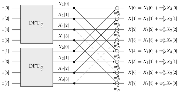
where $\underset{a}{\oplus}$ denotes the weigthed summation $g[k] + a \cdot h[k]$ of two signals whereby the weighted signal $h[k]$ is denoted by the arrow. The same decomposition is now applied to each of the DFTs of length $\frac{N}{2} = 4$ resulting in two DFTs of length $\frac{N}{4} = 2$
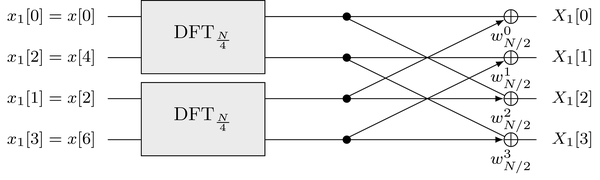
where $w_\frac{N}{2}^0 = w_N^0$, $w_\frac{N}{2}^1 = w_N^2$, $w_\frac{N}{2}^2 = w_N^4$ und $w_\frac{N}{2}^3 = w_N^6$. The resulting DFTs of length $2$ can be realized by
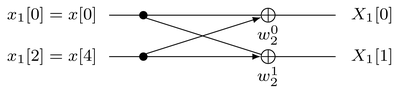
where $w_2^0 = 1$ und $w_2^1 = -1$. Combining the decompositions yields the overall flow diagram of the FFT for $N=8$
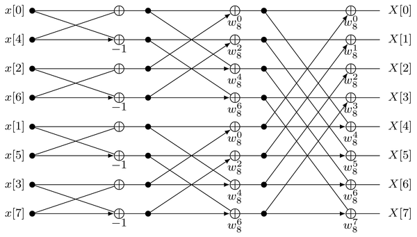
Further optimizations can be applied by noting that various common terms exist and that a sign reversal requires to swap only one bit in common representations of floating point numbers.
Benchmark
The radix-2 DIT algorithm presented above can only be applied to lengths $N = 2^w$ which are powers of two. Similar and other principles can be applied to derive efficient algorithms for other cases. A wide variety of implemented FFTs is available for many hardware platforms. Their computational efficiency depends heavily on the particular algorithm and hardware used. In the following the performance of the numpy.fft function is evaluated by comparing the execution times of a DFT realized by matrix/vector multiplication with the FFT algorithm. Note that the execution of the following cell may take some time.
import matplotlib.pyplot as plt
import numpy as np
import timeit
%matplotlib inline

n = np.arange(14)  # lengths = 2**n to evaluate
reps = 100  # number of repetitions per measurement

# measure execution times
gain = np.zeros(len(n))
for N in n:
    length = 2**N
    # setup environment for timeit
    tsetup = 'import numpy as np; from scipy.linalg import dft;  \
            x=np.random.randn(%d)+1j*np.random.randn(%d); F = dft(%d)' % (length, length, length)
    # DFT
    tc = timeit.timeit('np.matmul(F, x)', setup=tsetup, number=reps)
    # FFT
    tf = timeit.timeit('np.fft.fft(x)', setup=tsetup, number=reps)
    # gain by using the FFT
    gain[N] = tc/tf

# show the results
plt.barh(n, gain, log=True)
plt.plot([1, 1], [-1, n[-1]+1], 'r-')
plt.yticks(n, 2**n)
plt.xlabel('Gain of FFT')
plt.ylabel('Length $N$')
plt.title('Ratio of execution times between DFT and FFT')
plt.grid()
Exercise
- For which lengths $N$ is the FFT algorithm faster than the direct computation of the DFT?
- Why is it slower below a given length $N$?
- Does the trend of the gain follow the expected numerical complexity of the radix-2 FFT algorithm?
Copyright
This notebook is provided as Open Educational Resource. Feel free to use the notebook for your own purposes. The text is licensed under Creative Commons Attribution 4.0, the code of the IPython examples under the MIT license. Please attribute the work as follows: Sascha Spors, Continuous- and Discrete-Time Signals and Systems - Theory and Computational Examples.